Optimization Tutorial
Trey V. Wenger (c) July 2025
Here we demonstrate how to optimize the number of cloud components in a HFSRatioModel model.
[1]:
# General imports
import time

import matplotlib.pyplot as plt
import arviz as az
import pandas as pd
import numpy as np
import pymc as pm

import pytensor
print("pytensor version:", pytensor.__version__)

print("pymc version:", pm.__version__)
print("arviz version:", az.__version__)

import bayes_spec
print("bayes_spec version:", bayes_spec.__version__)

import bayes_hfs
print("bayes_hfs version:", bayes_hfs.__version__)

# Notebook configuration
pd.options.display.max_rows = None
pytensor version: 2.30.3
pymc version: 5.22.0
arviz version: 0.22.0dev
bayes_spec version: 1.9.0
bayes_hfs version: 1+0.gc6f9e00.dirty
Preparing Molecule Data
[2]:
from bayes_hfs import get_molecule_data, supplement_molecule_data
import pickle

try:
    all_mol_data_12CN, all_mol_metadata_12CN = get_molecule_data("CN, v=0,1", fmin=100.0, fmax=200.0)
    with open("mol_data_12CN.pkl", "wb") as f:
        pickle.dump(all_mol_data_12CN, f)
    with open("mol_metadata_12CN.pkl", "wb") as f:
        pickle.dump(all_mol_metadata_12CN, f)
except:
    with open("mol_data_12CN.pkl", "rb") as f:
        all_mol_data_12CN = pickle.load(f)
    with open("mol_metadata_12CN.pkl", "rb") as f:
        all_mol_metadata_12CN = pickle.load(f)

# Keep only Kl = 0 transitions
all_mol_data_12CN = all_mol_data_12CN[all_mol_data_12CN["Kl"] == 0]

# Add GLO
all_mol_data_12CN["GLO"] = 2 * all_mol_data_12CN["F1l"]

try:
    all_mol_data_13CN, all_mol_metadata_13CN = get_molecule_data("C-13-N", fmin=100.0, fmax=200.0)
    with open("mol_data_13CN.pkl", "wb") as f:
        pickle.dump(all_mol_data_13CN, f)
    with open("mol_metadata_13CN.pkl", "wb") as f:
        pickle.dump(all_mol_metadata_13CN, f)
except:
    with open("mol_data_13CN.pkl", "rb") as f:
        all_mol_data_13CN = pickle.load(f)
    with open("mol_metadata_13CN.pkl", "rb") as f:
        all_mol_metadata_13CN = pickle.load(f)

# Add GLO
all_mol_data_13CN["GLO"] = 2 * all_mol_data_13CN["F1l"] + 1

mol_data_12CN = supplement_molecule_data(all_mol_data_12CN, all_mol_metadata_12CN)
mol_data_13CN = supplement_molecule_data(all_mol_data_13CN, all_mol_metadata_13CN)
Model Definition and Simulated Data
[3]:
from bayes_spec import SpecData
from bayes_hfs import HFSRatioModel

# spectral axis definition
freq_axis_12CN_1 = np.arange(113110.0, 113200.0, 0.2) # MHz
freq_axis_12CN_2 = np.arange(113470.0, 113530.0, 0.2) # MHz
freq_axis_13CN_1 = np.arange(108620.0, 108670.0, 0.2) # MHz
freq_axis_13CN_2 = np.arange(108770.0, 108810.0, 0.2) # MHz

# data noise can either be a scalar (assumed constant noise across the spectrum)
# or an array of the same length as the data
noise = 0.001 # K

# brightness data. In this case, we just throw in some random data for now
# since we are only doing this in order to simulate some actual data.
brightness_data_12CN_1 = noise * np.random.randn(len(freq_axis_12CN_1)) # K
brightness_data_12CN_2 = noise * np.random.randn(len(freq_axis_12CN_2)) # K
brightness_data_13CN_1 = noise * np.random.randn(len(freq_axis_13CN_1)) # K
brightness_data_13CN_2 = noise * np.random.randn(len(freq_axis_13CN_2)) # K

# CNRatioModel expects observation names to contain either "12CN" or "13CN"
observation_12CN_1 = SpecData(
    freq_axis_12CN_1,
    brightness_data_12CN_1,
    noise,
    xlabel=r"LSRK Frequency (MHz)",
    ylabel=r"CN $T_B$ (K)",
)
observation_12CN_2 = SpecData(
    freq_axis_12CN_2,
    brightness_data_12CN_2,
    noise,
    xlabel=r"LSRK Frequency (MHz)",
    ylabel=r"CN $T_B$ (K)",
)
observation_13CN_1 = SpecData(
    freq_axis_13CN_1,
    brightness_data_13CN_1,
    noise,
    xlabel=r"LSRK Frequency (MHz)",
    ylabel=r"$^{13}$CN $T_B$ (K)",
)
observation_13CN_2 = SpecData(
    freq_axis_13CN_2,
    brightness_data_13CN_2,
    noise,
    xlabel=r"LSRK Frequency (MHz)",
    ylabel=r"$^{13}$CN $T_B$ (K)",
)
dummy_data = {
    "12CN-1": observation_12CN_1,
    "12CN-2": observation_12CN_2,
    "13CN-1": observation_13CN_1,
    "13CN-2": observation_13CN_2,
}

# association each dataset with the related species
mol_keys = {
    "12CN": ["12CN-1", "12CN-2"],
    "13CN": ["13CN-1", "13CN-2"],
}
[4]:
from bayes_hfs import HFSRatioModel
from bayes_hfs import physics

# Initialize and define the model
n_clouds = 3 # number of cloud components
baseline_degree = 0 # polynomial baseline degree
model = HFSRatioModel(
    mol_data_12CN, # molecular data for species 1
    mol_data_13CN, # molecular data for species 2
    mol_keys, # dataset association
    dummy_data,
    bg_temp = 2.7, # assumed background temperature (K)
    Beff = 1.0, # beam efficiency
    Feff = 1.0, # forward efficiency
    n_clouds=n_clouds,
    baseline_degree=baseline_degree,
    seed=1234,
    verbose=True
)
model.add_priors(
    prior_log10_Ntot1 = [13.5, 0.5], # mean and width of log10 total column density prior of first species (cm-2)
    prior_ratio = 0.1, # width of the column density ratio between the second and first species
    prior_fwhm2 = 1.0, # width of FWHM^2 prior (km2 s-2)
    prior_velocity = [-3.0, 3.0], # upper and lower limit of velocity prior (km/s)
    prior_log10_Tex_CTEX = [0.75, 0.25], # mean and width of log10 CTEX excitation temperature prior (K)
    assume_CTEX1 = False, # do not assume CTEX for the first species
    assume_CTEX2 = False, # assume CTEX for the second species for speed
    prior_log10_CTEX_variance = [-4.0, 1.0], # offset and width of log10 CTEX variance prior
    clip_weights = 1.0e-9, # clip statistical weights between [clip_weights, 1-clip_weights]
    clip_tau = -10.0, # clip optical depths below to prevent masers
    prior_fwhm_L = None, # assume Gaussian line profile
    prior_baseline_coeffs = None, # use default baseline priors
)
model.add_likelihood()

sim_params = {
    "log10_Ntot_12CN": np.array([13.8, 13.9, 14.0]),
    "ratio": np.array([1.0/65.0, 1.0/60.0, 1.0/55.0]),
    "fwhm2": np.array([1.0, 1.25, 1.5])**2.0,
    "velocity": [-2.0, 0.0, 2.5],
    "log10_Tex_CTEX": np.log10([4.46, 3.98, 3.16]),
    "log10_CTEX_variance": np.array([-1.5, -2.0, -3.0]),
    "baseline_12CN-1_norm": [0.0],
    "baseline_12CN-2_norm": [0.0],
    "baseline_13CN-1_norm": [0.0],
    "baseline_13CN-2_norm": [0.0],
}

CTEX_weights_12CN = physics.calc_stat_weight(
    model.mol1_data["states"]["deg"][None, :],
    model.mol1_data["states"]["E"][None, :],
    10.0 ** sim_params["log10_Tex_CTEX"][:, None],
).eval()

CTEX_concentration_12CN = (
    len(model.mol1_data["states"]["state"])
    * CTEX_weights_12CN
    / 10.0**sim_params["log10_CTEX_variance"][:, None]
)

from scipy.stats import dirichlet

sim_params["weights_12CN"] = np.stack([
    dirichlet(CTEX_concentration_12CN[i]).rvs()[0] for i in range(n_clouds)
])

# add derived quantities to sim_params
for key in model.cloud_deterministics:
    if key not in sim_params.keys():
        sim_params[key] = model.model[key].eval(sim_params, on_unused_input="ignore")

# Evaluate and save simulated observations
sim_12CN_1 = model.model["12CN-1"].eval(sim_params, on_unused_input="ignore")
sim_12CN_2 = model.model["12CN-2"].eval(sim_params, on_unused_input="ignore")
sim_13CN_1 = model.model["13CN-1"].eval(sim_params, on_unused_input="ignore")
sim_13CN_2 = model.model["13CN-2"].eval(sim_params, on_unused_input="ignore")

# pack simulated data
observation_12CN_1 = SpecData(
    freq_axis_12CN_1,
    sim_12CN_1,
    noise,
    xlabel=r"LSRK Frequency (MHz)",
    ylabel=r"CN $T_B$ (K)",
)
observation_12CN_2 = SpecData(
    freq_axis_12CN_2,
    sim_12CN_2,
    noise,
    xlabel=r"LSRK Frequency (MHz)",
    ylabel=r"CN $T_B$ (K)",
)
observation_13CN_1 = SpecData(
    freq_axis_13CN_1,
    sim_13CN_1,
    noise,
    xlabel=r"LSRK Frequency (MHz)",
    ylabel=r"$^{13}$CN $T_B$ (K)",
)
observation_13CN_2 = SpecData(
    freq_axis_13CN_2,
    sim_13CN_2,
    noise,
    xlabel=r"LSRK Frequency (MHz)",
    ylabel=r"$^{13}$CN $T_B$ (K)",
)
data = {
    "12CN-1": observation_12CN_1,
    "12CN-2": observation_12CN_2,
    "13CN-1": observation_13CN_1,
    "13CN-2": observation_13CN_2,
}
[5]:
sim_params
[5]:
{'log10_Ntot_12CN': array([13.8, 13.9, 14. ]),
 'ratio': array([0.01538462, 0.01666667, 0.01818182]),
 'fwhm2': array([1.    , 1.5625, 2.25  ]),
 'velocity': [-2.0, 0.0, 2.5],
 'log10_Tex_CTEX': array([0.64933486, 0.59988307, 0.49968708]),
 'log10_CTEX_variance': array([-1.5, -2. , -3. ]),
 'baseline_12CN-1_norm': [0.0],
 'baseline_12CN-2_norm': [0.0],
 'baseline_13CN-1_norm': [0.0],
 'baseline_13CN-2_norm': [0.0],
 'weights_12CN': array([[0.18099997, 0.35774445, 0.05141127, 0.10060146, 0.04239329,
         0.11086714, 0.15598241],
        [0.18391739, 0.37538564, 0.05147776, 0.0953406 , 0.04756006,
         0.09716964, 0.14914891],
        [0.22015952, 0.43069068, 0.03831167, 0.07664031, 0.03802426,
         0.07752001, 0.11865354]]),
 'log10_Ntot_13CN': array([11.98708664, 12.12184875, 12.25963731]),
 'CTEX_weights_12CN': array([[1.99954842, 4.        , 0.59193533, 1.18327051, 0.58954346,
         1.17923313, 1.76919492],
        [1.99949396, 4.        , 0.51109864, 1.02161662, 0.5087849 ,
         1.01771121, 1.52690069],
        [1.99936267, 4.        , 0.35871387, 0.71691448, 0.35666979,
         0.71346443, 1.07049146]]),
 'Tex_12CN': array([[6.62377784, 4.84728125, 3.18024483],
        [7.29549498, 5.1227256 , 3.24392405],
        [3.48460532, 4.06018147, 3.16334071],
        [3.66223901, 4.2517178 , 3.22631454],
        [3.26304903, 3.72315005, 2.96168302],
        [3.77468031, 4.02382954, 3.04074123],
        [2.70675076, 4.08302572, 3.14052123],
        [3.41789579, 3.88317284, 3.01669258],
        [2.81252526, 4.2761819 , 3.20240169]]),
 'tau_12CN': array([[0.02524333, 0.0360111 , 0.06420367],
        [0.17973349, 0.2691383 , 0.50431054],
        [0.28473286, 0.31504016, 0.51418762],
        [0.33573084, 0.37674563, 0.64106031],
        [0.38104257, 0.42733998, 0.68628587],
        [0.88301926, 1.03135861, 1.74637405],
        [0.32083078, 0.32311411, 0.53005213],
        [0.26725006, 0.30419385, 0.50807069],
        [0.03592579, 0.03636557, 0.06221058]]),
 'tau_total_12CN': array([2.71350897, 3.11930731, 5.25675546]),
 'TR_12CN': array([[4.27597848, 2.62918409, 1.20296471],
        [4.91419543, 2.87859882, 1.25318148],
        [1.44740238, 1.93265667, 1.18910571],
        [1.59417095, 2.09880298, 1.23863245],
        [1.26436858, 1.64130685, 1.0295351 ],
        [1.68461726, 1.89689066, 1.09001642],
        [0.8404223 , 1.94780861, 1.16743383],
        [1.38876463, 1.77628294, 1.07132523],
        [0.9174165 , 2.11549053, 1.21586649]]),
 'CTEX_weights_13CN': array([[3.        , 0.99376119, 2.9815721 , 4.9699281 , 0.92851903,
         0.31070072, 0.93202191, 1.55316693, 0.30874373, 0.92620269,
         1.54373121, 0.92472116, 1.54142752, 2.15832747],
        [3.        , 0.9930114 , 2.9793573 , 4.96631358, 0.80605378,
         0.26984676, 0.80946217, 1.34890613, 0.26794283, 0.80380078,
         1.33972638, 0.80236011, 1.3374862 , 1.87280054],
        [3.        , 0.9912059 , 2.9740239 , 4.95760931, 0.57313394,
         0.192086  , 0.57618799, 0.96013626, 0.19038061, 0.57111701,
         0.95191395, 0.56982806, 0.94990964, 1.33015962]]),
 'Tex_13CN': array([[3.63387014, 4.0123908 , 3.08464866],
        [3.83675886, 4.4342716 , 3.08229104],
        [3.84009247, 3.76818165, 3.2042096 ],
        [3.74209719, 4.19126825, 3.15773939],
        [4.66544699, 3.82749742, 3.11567771],
        [4.52148561, 4.26470704, 3.07173897],
        [5.00127202, 4.48112345, 3.08933137],
        [5.39889112, 4.17955656, 3.20886035],
        [5.20750875, 4.7045325 , 3.16240343],
        [4.0212438 , 5.15561858, 3.02750414],
        [4.02487718, 4.28049286, 3.14440333],
        [3.89187731, 3.60468882, 2.9993573 ],
        [4.17098129, 4.06799019, 3.15767616],
        [4.19325594, 3.19195589, 3.24091144],
        [4.12801426, 3.40738764, 3.11165721],
        [4.93507743, 4.35670617, 3.05954754],
        [4.05618042, 4.56249   , 3.11278043],
        [4.01553487, 3.74768332, 3.06805292],
        [3.95529061, 4.28992818, 3.1329999 ],
        [4.40618018, 3.92832745, 3.12736718],
        [4.18768408, 4.81107389, 3.18901639],
        [4.46192129, 4.46628177, 3.31607163],
        [4.2783927 , 4.38690557, 3.08338147],
        [4.33093502, 5.06851471, 3.26663988],
        [5.75698581, 4.81377011, 3.1490468 ],
        [4.38657499, 4.66567441, 3.10011369],
        [4.41108682, 3.55311919, 3.17987158],
        [4.33931568, 3.82058713, 3.05597262]]),
 'tau_13CN': array([[6.91016104e-05, 8.62078555e-05, 1.62414632e-04],
        [8.13865602e-05, 1.16170996e-04, 1.98952714e-04],
        [3.17002408e-05, 4.90748819e-05, 7.63535671e-05],
        [1.47575919e-04, 1.80064378e-04, 3.49181577e-04],
        [7.71761587e-05, 1.30964896e-04, 2.07535796e-04],
        [2.17990215e-04, 2.89708089e-04, 5.72893422e-04],
        [2.47769861e-04, 3.43972966e-04, 6.84887892e-04],
        [7.31425101e-04, 1.29197271e-03, 2.11177097e-03],
        [1.54527530e-03, 2.10941210e-03, 4.34270099e-03],
        [8.23550053e-04, 9.98210130e-04, 2.27788743e-03],
        [2.47848809e-03, 3.32640756e-03, 6.75966969e-03],
        [1.07463295e-03, 1.45504622e-03, 2.63385994e-03],
        [1.13999026e-03, 1.77112462e-03, 2.87381935e-03],
        [8.52386088e-04, 1.47913347e-03, 2.13240347e-03],
        [7.37813449e-04, 1.23676746e-03, 1.86095314e-03],
        [3.77625764e-03, 5.59115358e-03, 1.15866992e-02],
        [3.38711307e-03, 4.11006613e-03, 8.37106802e-03],
        [9.41168554e-04, 1.25350083e-03, 2.32747602e-03],
        [6.96307786e-03, 8.62039131e-03, 1.69549542e-02],
        [3.35612901e-03, 5.45424590e-03, 8.73289194e-03],
        [1.64511631e-03, 1.99815187e-03, 4.08158818e-03],
        [1.15227317e-03, 1.76718272e-03, 2.94828359e-03],
        [1.25328535e-03, 1.59472409e-03, 3.19246242e-03],
        [8.79240704e-05, 1.04039577e-04, 2.20310632e-04],
        [1.16316006e-05, 1.78720936e-05, 3.86220767e-05],
        [2.82315246e-04, 3.78176622e-04, 8.07986128e-04],
        [7.29919449e-05, 1.12072231e-04, 2.07457051e-04],
        [1.98775501e-04, 2.92855454e-04, 5.68804114e-04]]),
 'tau_total_13CN': array([0.03338432, 0.04615867, 0.08728389]),
 'TR_13CN': array([[1.63769168, 1.96304246, 1.18617309],
        [1.8108763 , 2.33556625, 1.184289  ],
        [1.8136662 , 1.75193053, 1.28186856],
        [1.72943434, 2.11957112, 1.24428871],
        [2.54293543, 1.80263014, 1.21062722],
        [2.41313236, 2.18424104, 1.17551796],
        [2.84302083, 2.37219693, 1.18580068],
        [3.20891541, 2.10436621, 1.28139781],
        [3.03194919, 2.5728406 , 1.24385719],
        [1.96259901, 2.98090426, 1.13437175],
        [1.96568165, 2.19018492, 1.22695166],
        [1.85033635, 1.60534487, 1.11222735],
        [2.09347408, 2.00319904, 1.23749058],
        [2.11306356, 1.26499364, 1.30450211],
        [2.0557196 , 1.44064407, 1.20074399],
        [2.77867001, 2.25756471, 1.15937469],
        [1.99268517, 2.44131639, 1.20148997],
        [1.9572337 , 1.72631391, 1.16600468],
        [1.90319648, 2.19642801, 1.21615459],
        [2.29963139, 1.87982136, 1.21163864],
        [2.10608725, 2.66372918, 1.26092144],
        [2.3491845 , 2.35308013, 1.3637902 ],
        [2.18598191, 2.28226144, 1.17653557],
        [2.23236108, 2.89813924, 1.32336919],
        [3.53239079, 2.66305005, 1.2265218 ],
        [2.2756973 , 2.52556554, 1.1848887 ],
        [2.29749236, 1.55445369, 1.24843537],
        [2.23371459, 1.78103118, 1.15001426]])}
Optimize
We use the Optimize class for optimization.
[6]:
from bayes_spec import Optimize
from bayes_hfs import HFSRatioModel

# Initialize optimizer
opt = Optimize(
    HFSRatioModel,
    mol_data_12CN, # molecular data for species 1
    mol_data_13CN, # molecular data for species 2
    mol_keys, # dataset association
    data,
    bg_temp = 2.7, # assumed background temperature (K)
    Beff = 1.0, # beam efficiency
    Feff = 1.0, # forward efficiency
    max_n_clouds=5,
    baseline_degree=baseline_degree,
    seed=1234,
    verbose=True
)

# Define each model
opt.add_priors(
    prior_log10_Ntot1 = [13.5, 0.5], # mean and width of log10 total column density prior of first species (cm-2)
    prior_ratio = 0.1, # width of the column density ratio between the second and first species
    prior_fwhm2 = 1.0, # width of FWHM^2 prior (km2 s-2)
    prior_velocity = [-3.0, 3.0], # upper and lower limit of velocity prior (km/s)
    prior_log10_Tex_CTEX = [0.75, 0.25], # mean and width of log10 CTEX excitation temperature prior (K)
    assume_CTEX1 = False, # do not assume CTEX for the first species
    assume_CTEX2 = True, # assume CTEX for the second species for speed
    prior_log10_CTEX_variance = [-4.0, 1.0], # offset and width of log10 CTEX variance prior
    clip_weights = 1.0e-9, # clip statistical weights between [clip_weights, 1-clip_weights]
    clip_tau = -10.0, # clip optical depths below to prevent masers
    prior_fwhm_L = None, # assume Gaussian line profile
    prior_baseline_coeffs = None, # use default baseline priors
)
opt.add_likelihood()
Optimize has created max_n_clouds models, where opt.models[1] has n_clouds=1, opt.models[2] has n_clouds=2, etc.
[7]:
print(opt.models[4])
print(opt.models[4].n_clouds)
<bayes_hfs.hfs_ratio_model.HFSRatioModel object at 0x7bc38d9b2650>
4
By default (approx=True), the optimization algorithm first loops over every model and approximates the posterior distribution using variational inference. This is generally a bad idea, since VI is only an approximation and tends to struggle with complex models. Instead we use approx=False to sample every model with MCMC. This is slower but more robust.
We can supply arguments to fit and sample via dictionaries. Whichever model is the first to have a BIC within bic_threshold of the minimum BIC is the “best” model. The algorithm will terminate early if successive models have increasing BICs or fail to converge.
[8]:
fit_kwargs = {
    "rel_tolerance": 0.01,
    "abs_tolerance": 0.01,
    "learning_rate": 0.001,
}
sample_kwargs = {
    "chains": 8,
    "cores": 8,
    "n_init": 200_000,
    "init_kwargs": fit_kwargs,
    "nuts_kwargs": {"target_accept": 0.9},
}
solve_kwargs = {
    "init_params": "random_from_data",
    "n_init": 10,
    "max_iter": 1_000,
    "kl_div_threshold": 0.1,
}
opt.optimize(
    bic_threshold=10.0,
    sample_kwargs=sample_kwargs,
    fit_kwargs=fit_kwargs,
    solve_kwargs=solve_kwargs,
    approx=False,
    start_spread = {"velocity_norm": [0.1, 0.9]},
)
Null hypothesis BIC = 1.132e+07
Sampling n_cloud = 1 posterior...
Initializing NUTS using custom advi+adapt_diag strategy
Convergence achieved at 41000
Interrupted at 40,999 [20%]: Average Loss = 1.8552e+17
Multiprocess sampling (8 chains in 8 jobs)
NUTS: [baseline_12CN-1_norm, baseline_12CN-2_norm, baseline_13CN-1_norm, baseline_13CN-2_norm, log10_Ntot_12CN_norm, ratio_norm, fwhm2_norm, velocity_norm, log10_Tex_CTEX_norm, log10_CTEX_variance_norm, weights_12CN_norm]
Sampling 8 chains for 1_000 tune and 1_000 draw iterations (8_000 + 8_000 draws total) took 1162 seconds.
Adding log-likelihood to trace
GMM converged to unique solution
n_cloud = 1 solution = 0 BIC = 2.335e+06

Sampling n_cloud = 2 posterior...
Initializing NUTS using custom advi+adapt_diag strategy
Convergence achieved at 45400
Interrupted at 45,399 [22%]: Average Loss = 7.3459e+19
Multiprocess sampling (8 chains in 8 jobs)
NUTS: [baseline_12CN-1_norm, baseline_12CN-2_norm, baseline_13CN-1_norm, baseline_13CN-2_norm, log10_Ntot_12CN_norm, ratio_norm, fwhm2_norm, velocity_norm, log10_Tex_CTEX_norm, log10_CTEX_variance_norm, weights_12CN_norm]
Sampling 8 chains for 1_000 tune and 1_000 draw iterations (8_000 + 8_000 draws total) took 5737 seconds.
Adding log-likelihood to trace
GMM converged to unique solution
n_cloud = 2 solution = 0 BIC = 6.866e+05

Sampling n_cloud = 3 posterior...
Initializing NUTS using custom advi+adapt_diag strategy
Convergence achieved at 56200
Interrupted at 56,199 [28%]: Average Loss = 4.8623e+28
Multiprocess sampling (8 chains in 8 jobs)
NUTS: [baseline_12CN-1_norm, baseline_12CN-2_norm, baseline_13CN-1_norm, baseline_13CN-2_norm, log10_Ntot_12CN_norm, ratio_norm, fwhm2_norm, velocity_norm, log10_Tex_CTEX_norm, log10_CTEX_variance_norm, weights_12CN_norm]
Sampling 8 chains for 1_000 tune and 1_000 draw iterations (8_000 + 8_000 draws total) took 1155 seconds.
Adding log-likelihood to trace
There were 990 divergences in converged chains.
GMM converged to unique solution
6 of 8 chains appear converged.
n_cloud = 3 solution = 0 BIC = -1.277e+04

Sampling n_cloud = 4 posterior...
Initializing NUTS using custom advi+adapt_diag strategy
Convergence achieved at 65600
Interrupted at 65,599 [32%]: Average Loss = 7.3701e+21
Multiprocess sampling (8 chains in 8 jobs)
NUTS: [baseline_12CN-1_norm, baseline_12CN-2_norm, baseline_13CN-1_norm, baseline_13CN-2_norm, log10_Ntot_12CN_norm, ratio_norm, fwhm2_norm, velocity_norm, log10_Tex_CTEX_norm, log10_CTEX_variance_norm, weights_12CN_norm]
Sampling 8 chains for 1_000 tune and 1_000 draw iterations (8_000 + 8_000 draws total) took 5104 seconds.
Adding log-likelihood to trace
There were 330 divergences in converged chains.
GMM found 3 unique solutions
Solution 0: chains [np.int64(0), np.int64(1)]
Solution 1: chains [np.int64(3), np.int64(6), np.int64(7)]
Solution 2: chains [np.int64(4), np.int64(5)]
7 of 8 chains appear converged.
n_cloud = 4 solution = 0 BIC = -1.267e+04
n_cloud = 4 solution = 1 BIC = -1.267e+04
n_cloud = 4 solution = 2 BIC = -1.267e+04

Stopping criteria met.
Sampling n_cloud = 5 posterior...
Initializing NUTS using custom advi+adapt_diag strategy
Convergence achieved at 76300
Interrupted at 76,299 [38%]: Average Loss = 7.9475e+24
Multiprocess sampling (8 chains in 8 jobs)
NUTS: [baseline_12CN-1_norm, baseline_12CN-2_norm, baseline_13CN-1_norm, baseline_13CN-2_norm, log10_Ntot_12CN_norm, ratio_norm, fwhm2_norm, velocity_norm, log10_Tex_CTEX_norm, log10_CTEX_variance_norm, weights_12CN_norm]
Sampling 8 chains for 1_000 tune and 1_000 draw iterations (8_000 + 8_000 draws total) took 6427 seconds.
Adding log-likelihood to trace
There were 271 divergences in converged chains.
No solution found!
0 of 8 chains appear converged.

Stopping criteria met.
Stopping early.
[9]:
opt.best_model.n_clouds
[9]:
3
[12]:
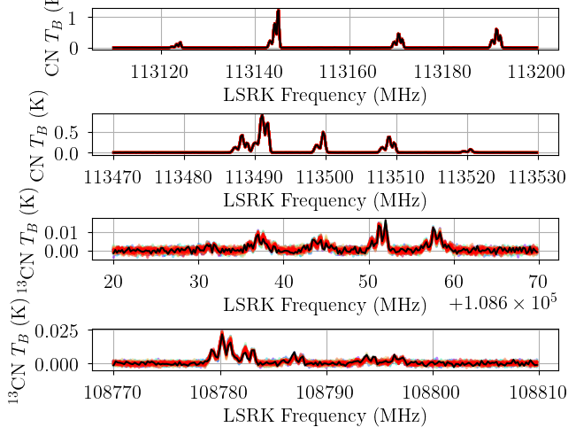
from bayes_spec.plots import plot_predictive

posterior = opt.best_model.sample_posterior_predictive(
    thin=100, # keep one in {thin} posterior samples
)
axes = plot_predictive(opt.best_model.data, posterior.posterior_predictive)
Sampling: [12CN-1, 12CN-2, 13CN-1, 13CN-2]
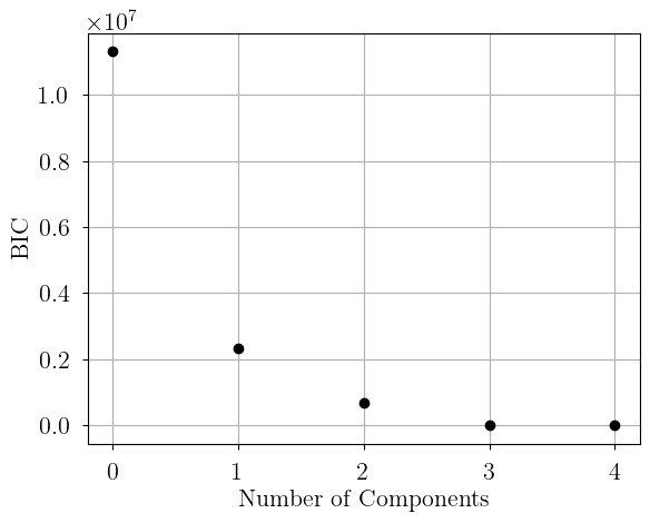
[13]:
plt.plot(opt.bics.keys(), opt.bics.values(), 'ko')
plt.xlabel("Number of Components")
plt.ylabel("BIC")
[13]:
Text(0, 0.5, 'BIC')
[ ]: