HFSModel Tutorial
Trey V. Wenger (c) July 2025
Here we demonstrate the basic features of the HFSModel model. The HFSModel models hyperfine spectral structure including non-CTEX effects. Please review the bayes_spec documentation and tutorials for a more thorough description of the steps outlined in this tutorial: https://bayes-spec.readthedocs.io/en/stable/index.html
[1]:
# General imports
import time

import matplotlib.pyplot as plt
import arviz as az
import pandas as pd
import numpy as np
import pymc as pm

print("pymc version:", pm.__version__)
print("arviz version:", az.__version__)

import bayes_spec
print("bayes_spec version:", bayes_spec.__version__)

import bayes_hfs
print("bayes_hfs version:", bayes_hfs.__version__)

# Notebook configuration
pd.options.display.max_rows = None
pymc version: 5.22.0
arviz version: 0.22.0dev
bayes_spec version: 1.9.0
bayes_hfs version: 1+0.gc6f9e00.dirty
Preparing Molecule Data
Here we model the hyperfine structure of CN transitions to the ground rotational state. We must first manually identify the transitions of interest and calculate the lower state degeneracies. (N.B., if anyone knows how to derive the lower state degeneracies programmatically from the information returned by CDMS, please let me know!)
[2]:
from bayes_hfs import get_molecule_data, supplement_molecule_data
import pickle

try:
    all_mol_data_12CN, all_mol_metadata_12CN = get_molecule_data("CN, v=0,1", fmin=100.0, fmax=200.0)
    with open("mol_data_12CN.pkl", "wb") as f:
        pickle.dump(all_mol_data_12CN, f)
    with open("mol_metadata_12CN.pkl", "wb") as f:
        pickle.dump(all_mol_metadata_12CN, f)
except:
    with open("mol_data_12CN.pkl", "rb") as f:
        all_mol_data_12CN = pickle.load(f)
    with open("mol_metadata_12CN.pkl", "rb") as f:
        all_mol_metadata_12CN = pickle.load(f)

all_mol_data_12CN.pprint_all()
    FREQ     ERR    LGINT   DR    ELO    GUP MOLWT TAG  QNFMT  Ju  Ku  vu F1u F2u F3u  Jl  Kl  vl F1l F2l F3l    name    Lab
    MHz      MHz   nm2 MHz       1 / cm        u
----------- ------ ------- --- --------- --- ----- ---- ----- --- --- --- --- --- --- --- --- --- --- --- --- --------- -----
 112101.656   0.05 -8.0612   2 2042.4216   2    26 5041   234   1   1   1   1  --  --   0   1   1   2  --  -- CN, v=0,1  True
 112128.989   0.05  -8.069   2 2042.4222   4    26 5041   234   1   1   1   2  --  --   0   1   1   1  --  -- CN, v=0,1  True
 112148.503   0.05 -7.9593   2 2042.4216   4    26 5041   234   1   1   1   2  --  --   0   1   1   2  --  -- CN, v=0,1  True
 112442.806   0.05 -7.9569   2 2042.4222   4    26 5041   234   1   1   2   2  --  --   0   1   1   1  --  -- CN, v=0,1  True
 112445.015   0.05 -7.5311   2 2042.4216   6    26 5041   234   1   1   2   3  --  --   0   1   1   2  --  -- CN, v=0,1  True
 112453.876   0.05 -8.0586   2 2042.4222   2    26 5041   234   1   1   2   1  --  --   0   1   1   1  --  -- CN, v=0,1  True
 112462.292   0.05 -8.0664   2 2042.4216   4    26 5041   234   1   1   2   2  --  --   0   1   1   2  --  -- CN, v=0,1  True
113123.3701 0.0058 -4.7118   2    0.0007   2    26 5041   234   1   0   1   1  --  --   0   0   1   1  --  -- CN, v=0,1 False
113144.1573 0.0057 -3.7989   2      -0.0   2    26 5041   234   1   0   1   1  --  --   0   0   1   2  --  -- CN, v=0,1 False
113170.4915 0.0039  -3.809   2    0.0007   4    26 5041   234   1   0   1   2  --  --   0   0   1   1  --  -- CN, v=0,1 False
113191.2787 0.0034 -3.6955   2      -0.0   4    26 5041   234   1   0   1   2  --  --   0   0   1   2  --  -- CN, v=0,1 False
113488.1202 0.0033 -3.6932   2    0.0007   4    26 5041   234   1   0   2   2  --  --   0   0   1   1  --  -- CN, v=0,1 False
113490.9702 0.0024 -3.2691   2      -0.0   6    26 5041   234   1   0   2   3  --  --   0   0   1   2  --  -- CN, v=0,1 False
113499.6443 0.0028 -3.7962   2    0.0007   2    26 5041   234   1   0   2   1  --  --   0   0   1   1  --  -- CN, v=0,1 False
113508.9074 0.0028 -3.8065   2      -0.0   4    26 5041   234   1   0   2   2  --  --   0   0   1   2  --  -- CN, v=0,1 False
113520.4315 0.0044  -4.709   2      -0.0   2    26 5041   234   1   0   2   1  --  --   0   0   1   2  --  -- CN, v=0,1 False
[3]:
# Keep only Kl = 0 transitions
all_mol_data_12CN = all_mol_data_12CN[all_mol_data_12CN["Kl"] == 0]

# Add GLO
all_mol_data_12CN["GLO"] = 2 * all_mol_data_12CN["F1l"]

all_mol_data_12CN.pprint_all()
    FREQ     ERR    LGINT   DR  ELO   GUP MOLWT TAG  QNFMT  Ju  Ku  vu F1u F2u F3u  Jl  Kl  vl F1l F2l F3l    name    Lab  GLO
    MHz      MHz   nm2 MHz     1 / cm       u
----------- ------ ------- --- ------ --- ----- ---- ----- --- --- --- --- --- --- --- --- --- --- --- --- --------- ----- ---
113123.3701 0.0058 -4.7118   2 0.0007   2    26 5041   234   1   0   1   1  --  --   0   0   1   1  --  -- CN, v=0,1 False   2
113144.1573 0.0057 -3.7989   2   -0.0   2    26 5041   234   1   0   1   1  --  --   0   0   1   2  --  -- CN, v=0,1 False   4
113170.4915 0.0039  -3.809   2 0.0007   4    26 5041   234   1   0   1   2  --  --   0   0   1   1  --  -- CN, v=0,1 False   2
113191.2787 0.0034 -3.6955   2   -0.0   4    26 5041   234   1   0   1   2  --  --   0   0   1   2  --  -- CN, v=0,1 False   4
113488.1202 0.0033 -3.6932   2 0.0007   4    26 5041   234   1   0   2   2  --  --   0   0   1   1  --  -- CN, v=0,1 False   2
113490.9702 0.0024 -3.2691   2   -0.0   6    26 5041   234   1   0   2   3  --  --   0   0   1   2  --  -- CN, v=0,1 False   4
113499.6443 0.0028 -3.7962   2 0.0007   2    26 5041   234   1   0   2   1  --  --   0   0   1   1  --  -- CN, v=0,1 False   2
113508.9074 0.0028 -3.8065   2   -0.0   4    26 5041   234   1   0   2   2  --  --   0   0   1   2  --  -- CN, v=0,1 False   4
113520.4315 0.0044  -4.709   2   -0.0   2    26 5041   234   1   0   2   1  --  --   0   0   1   2  --  -- CN, v=0,1 False   4
[4]:
mol_data_12CN = supplement_molecule_data(all_mol_data_12CN, all_mol_metadata_12CN)
print(mol_data_12CN.keys())
print("molecular weight (Daltons):", mol_data_12CN['mol_weight'])
print("transition frequency (MHz):", mol_data_12CN['freq'])
print("Einstein A coefficient (s-1):", mol_data_12CN['Aul'])
print("Relative intensities:", mol_data_12CN['relative_int'])
print("state info:", mol_data_12CN["states"])
print("upper state index:", mol_data_12CN["state_u_idx"])
print("lower state index:", mol_data_12CN["state_l_idx"])
print("upper state degeneracy:", mol_data_12CN["Gu"])
print("lower state degeneracy:", mol_data_12CN["Gl"])
dict_keys(['mol_weight', 'freq', 'Aul', 'relative_int', 'states', 'state_u_idx', 'state_l_idx', 'Gu', 'Gl'])
molecular weight (Daltons): 26
transition frequency (MHz): [113123.3701 113144.1573 113170.4915 113191.2787 113488.1202 113490.9702
 113499.6443 113508.9074 113520.4315]
Einstein A coefficient (s-1): [1.24997446e-06 1.02301076e-05 4.99866053e-06 6.49280964e-06
 6.54458098e-06 1.15851092e-05 1.03265758e-05 5.04267116e-06
 1.26251089e-06]
Relative intensities: [0.01204927 0.09859632 0.09632981 0.12510097 0.12576526 0.33393404
 0.0992112  0.09688593 0.0121272 ]
state info: {'state': [np.str_('0 0 1 1 -- --'), np.str_('0 0 1 2 -- --'), np.str_('1 0 1 1 -- --'), np.str_('1 0 1 2 -- --'), np.str_('1 0 2 1 -- --'), np.str_('1 0 2 2 -- --'), np.str_('1 0 2 3 -- --')], 'deg': array([2, 4, 2, 4, 2, 4, 6]), 'E': array([ 1.00714381e-03, -0.00000000e+00,  5.43007265e+00,  5.43233412e+00,
        5.44813096e+00,  5.44757789e+00,  5.44670753e+00])}
upper state index: [2, 2, 3, 3, 5, 6, 4, 5, 4]
lower state index: [0, 1, 0, 1, 0, 1, 0, 1, 1]
upper state degeneracy: [2 2 4 4 4 6 2 4 2]
lower state degeneracy: [2 4 2 4 2 4 2 4 4]
Simulating Data
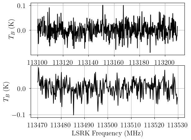
To test the model, we must simulate some data. We can do this with HFSModel, but we must pack a “dummy” data structure first. The observations can be named anything (e.g., “12CN-1” and “12CN-2” in this case).
[5]:
from bayes_spec import SpecData

# spectral axis definition
freq_axis_1 = np.arange(113100.0, 113210.0, 0.2) # MHz
freq_axis_2 = np.arange(113470.0, 113530.0, 0.2) # MHz

# data noise can either be a scalar (assumed constant noise across the spectrum)
# or an array of the same length as the data
noise = 0.03 # K

# brightness data. In this case, we just throw in some random data for now
# since we are only doing this in order to simulate some actual data.
brightness_data_1 = noise * np.random.randn(len(freq_axis_1)) # K
brightness_data_2 = noise * np.random.randn(len(freq_axis_2)) # K

# HFSModel datasets can be named anything, here we name them "12CN-1" and "12CN-2"
obs_1 = SpecData(
    freq_axis_1,
    brightness_data_1,
    noise,
    xlabel=r"LSRK Frequency (MHz)",
    ylabel=r"$T_B$ (K)",
)
obs_2 = SpecData(
    freq_axis_2,
    brightness_data_2,
    noise,
    xlabel=r"LSRK Frequency (MHz)",
    ylabel=r"$T_B$ (K)",
)
dummy_data = {"12CN-1": obs_1, "12CN-2": obs_2}

# Plot the simulated data
fig, axes = plt.subplots(2)
axes[0].plot(dummy_data["12CN-1"].spectral, dummy_data["12CN-1"].brightness, "k-")
axes[0].set_ylabel(dummy_data["12CN-1"].ylabel)
axes[1].plot(dummy_data["12CN-2"].spectral, dummy_data["12CN-2"].brightness, "k-")
axes[1].set_xlabel(dummy_data["12CN-2"].xlabel)
_ = axes[1].set_ylabel(dummy_data["12CN-2"].ylabel)
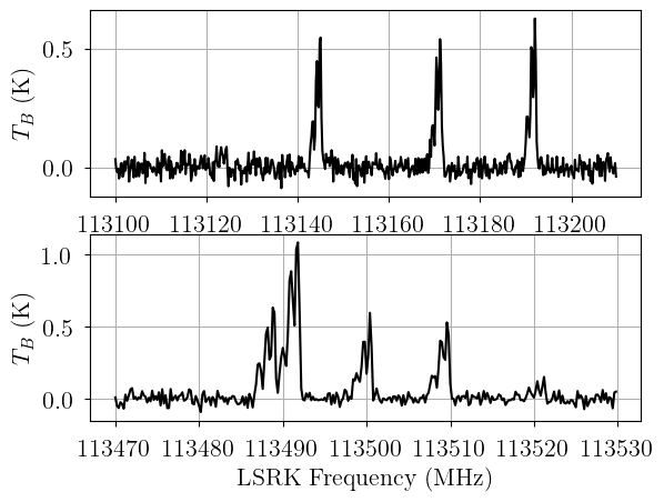
Now that we have a dummy data format, we can generate a simulated observation by evaluating the model for a given set of model parameters.
[6]:
from bayes_hfs import HFSModel

# Initialize and define the model
n_clouds = 3 # number of cloud components
baseline_degree = 0 # polynomial baseline degree
model = HFSModel(
    mol_data_12CN, # molecular data
    dummy_data,
    bg_temp = 2.7, # assumed background temperature (K)
    Beff = 1.0, # beam efficiency
    Feff = 1.0, # forward efficiency
    n_clouds=n_clouds,
    baseline_degree=baseline_degree,
    seed=1234,
    verbose=True
)
model.add_priors(
    prior_log10_Ntot = [13.5, 0.5], # mean and width of log10 total column density prior (cm-2)
    prior_fwhm2 = 1.0, # width of FWHM^2 prior (km2 s-2)
    prior_velocity = [-3.0, 3.0], # upper and lower limit of velocity prior (km/s)
    prior_log10_Tex_CTEX = [0.75, 0.25], # mean and width of log10 CTEX excitation temperature prior (K)
    assume_CTEX = True, # assume CTEX
    prior_log10_CTEX_variance = None, # ignored because CTEX
    clip_weights = 1.0e-9, # clip statistical weights between [clip_weights, 1-clip_weights]
    clip_tau = -10.0, # clip optical depths below to prevent masers
    prior_fwhm_L = None, # assume Gaussian line profile
    prior_baseline_coeffs = None, # use default baseline priors
)
model.add_likelihood()

sim_params = {
    "log10_Ntot": np.array([13.8, 13.9, 14.0]),
    "fwhm2": np.array([1.0, 1.25, 1.5])**2.0,
    "velocity": [-2.0, 0.0, 2.5],
    "log10_Tex_CTEX": np.log10([4.46, 3.98, 3.16]),
    "baseline_12CN-1_norm": [0.0],
    "baseline_12CN-2_norm": [0.0],
}

# add derived quantities to sim_params
for key in model.cloud_deterministics:
    if key not in sim_params.keys():
        sim_params[key] = model.model[key].eval(sim_params, on_unused_input="ignore")

# Evaluate and save simulated observations
sim_obs1 = model.model["12CN-1"].eval(sim_params, on_unused_input="ignore")
sim_obs2 = model.model["12CN-2"].eval(sim_params, on_unused_input="ignore")

# Plot the simulated data
fig, axes = plt.subplots(2)
axes[0].plot(dummy_data["12CN-1"].spectral, sim_obs1, "k-")
axes[0].set_ylabel(dummy_data["12CN-1"].ylabel)
axes[1].plot(dummy_data["12CN-2"].spectral, sim_obs2, "k-")
axes[1].set_xlabel(dummy_data["12CN-2"].xlabel)
_ = axes[1].set_ylabel(dummy_data["12CN-2"].ylabel)
[7]:
sim_params
[7]:
{'log10_Ntot': array([13.8, 13.9, 14. ]),
 'fwhm2': array([1.    , 1.5625, 2.25  ]),
 'velocity': [-2.0, 0.0, 2.5],
 'log10_Tex_CTEX': array([0.64933486, 0.59988307, 0.49968708]),
 'baseline_12CN-1_norm': [0.0],
 'baseline_12CN-2_norm': [0.0],
 'CTEX_weights': array([[1.99954842, 4.        , 0.59193533, 1.18327051, 0.58954346,
         1.17923313, 1.76919492],
        [1.99949396, 4.        , 0.51109864, 1.02161662, 0.5087849 ,
         1.01771121, 1.52690069],
        [1.99936267, 4.        , 0.35871387, 0.71691448, 0.35666979,
         0.71346443, 1.07049146]]),
 'Tex': array([4.46, 3.98, 3.16]),
 'tau': array([[0.02742294, 0.03901221, 0.06218552],
        [0.22442582, 0.31927704, 0.50895265],
        [0.21919336, 0.3118215 , 0.49702465],
        [0.28469915, 0.40501691, 0.6456038 ],
        [0.28578764, 0.40650805, 0.64778077],
        [0.75898784, 1.07962237, 1.72051429],
        [0.22543548, 0.32066093, 0.51097642],
        [0.22019236, 0.31321047, 0.49913295],
        [0.02756012, 0.03920245, 0.06247252]]),
 'tau_total': array([2.27370471, 3.23433194, 5.15464356]),
 'TR': array([[2.28305326, 1.86428157, 1.18701886],
        [2.28274737, 1.8639964 , 1.18678032],
        [2.28235989, 1.86363517, 1.18647818],
        [2.28205408, 1.86335008, 1.18623973],
        [2.27769048, 1.85928267, 1.18283893],
        [2.27764861, 1.85924365, 1.18280632],
        [2.2775212 , 1.85912491, 1.18270707],
        [2.27738515, 1.8589981 , 1.18260108],
        [2.27721589, 1.85884036, 1.18246924]])}
[8]:
# Now we pack the simulated spectrum into a new SpecData instance
obs_1 = SpecData(
    freq_axis_1,
    sim_obs1,
    noise,
    xlabel=r"LSRK Frequency (MHz)",
    ylabel=r"$T_B$ (K)",
)
obs_2 = SpecData(
    freq_axis_2,
    sim_obs2,
    noise,
    xlabel=r"LSRK Frequency (MHz)",
    ylabel=r"$T_B$ (K)",
)
data = {"12CN-1": obs_1, "12CN-2": obs_2}
Model Definition
Finally, with our model definition and (simulated) data in hand, we can explore the capabilities of HFSModel. Here we assume constant excitation temperature (CTEX).
[9]:
# Initialize and define the model
model = HFSModel(
    mol_data_12CN, # molecular data
    data,
    bg_temp = 2.7, # assumed background temperature (K)
    Beff = 1.0, # beam efficiency
    Feff = 1.0, # forward efficiency
    n_clouds=n_clouds,
    baseline_degree=baseline_degree,
    seed=1234,
    verbose=True
)
model.add_priors(
    prior_log10_Ntot = [13.5, 0.5], # mean and width of log10 total column density prior (cm-2)
    prior_fwhm2 = 1.0, # width of FWHM^2 prior (km2 s-2)
    prior_velocity = [-3.0, 3.0], # upper and lower limit of velocity prior (km/s)
    prior_log10_Tex_CTEX = [0.75, 0.25], # mean and width of log10 CTEX excitation temperature prior (K)
    assume_CTEX = True, # assume CTEX
    prior_log10_CTEX_variance = None, # ignored because CTEX
    clip_weights = 1.0e-9, # clip statistical weights between [clip_weights, 1-clip_weights]
    clip_tau = -10.0, # clip optical depths below to prevent masers
    prior_fwhm_L = None, # assume Gaussian line profile
    prior_baseline_coeffs = None, # use default baseline priors
)
model.add_likelihood()
[10]:
# Plot model graph
model.graph().render('hfs_model', format='png')
model.graph()
[10]:

[11]:
# model string representation
print(model.model.str_repr())
baseline_12CN-1_norm ~ Normal(0, 1)
baseline_12CN-2_norm ~ Normal(0, 1)
     log10_Ntot_norm ~ Normal(0, 1)
          fwhm2_norm ~ Gamma(0.5, f())
       velocity_norm ~ Beta(2, 2)
 log10_Tex_CTEX_norm ~ Normal(0, 1)
          log10_Ntot ~ Deterministic(f(log10_Ntot_norm))
               fwhm2 ~ Deterministic(f(fwhm2_norm))
            velocity ~ Deterministic(f(velocity_norm))
      log10_Tex_CTEX ~ Deterministic(f(log10_Tex_CTEX_norm))
        CTEX_weights ~ Deterministic(f(log10_Tex_CTEX_norm))
                 Tex ~ Deterministic(f(log10_Tex_CTEX_norm))
                 tau ~ Deterministic(f(log10_Ntot_norm, log10_Tex_CTEX_norm))
           tau_total ~ Deterministic(f(log10_Ntot_norm, log10_Tex_CTEX_norm))
                  TR ~ Deterministic(f(log10_Tex_CTEX_norm))
              12CN-1 ~ Normal(f(baseline_12CN-1_norm, log10_Tex_CTEX_norm, velocity_norm, fwhm2_norm, log10_Ntot_norm), <constant>)
              12CN-2 ~ Normal(f(baseline_12CN-2_norm, log10_Tex_CTEX_norm, velocity_norm, fwhm2_norm, log10_Ntot_norm), <constant>)
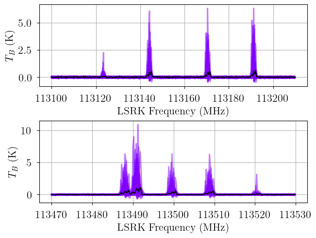
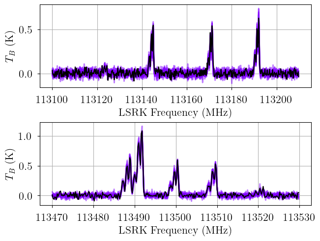
We check that our prior distributions are reasonable by drawing prior predictive checks. Each colored line is a simulated “observation” with parameters drawn from the prior distributions. You should check that these simulated observations at least somewhat overlap your actual observation (black line).
[12]:
from bayes_spec.plots import plot_predictive

# prior predictive check
prior = model.sample_prior_predictive(
    samples=1000,  # prior predictive samples
)
_ = plot_predictive(model.data, prior.prior_predictive.sel(draw=slice(None, None, 20)))
Sampling: [12CN-1, 12CN-2, baseline_12CN-1_norm, baseline_12CN-2_norm, fwhm2_norm, log10_Ntot_norm, log10_Tex_CTEX_norm, velocity_norm]
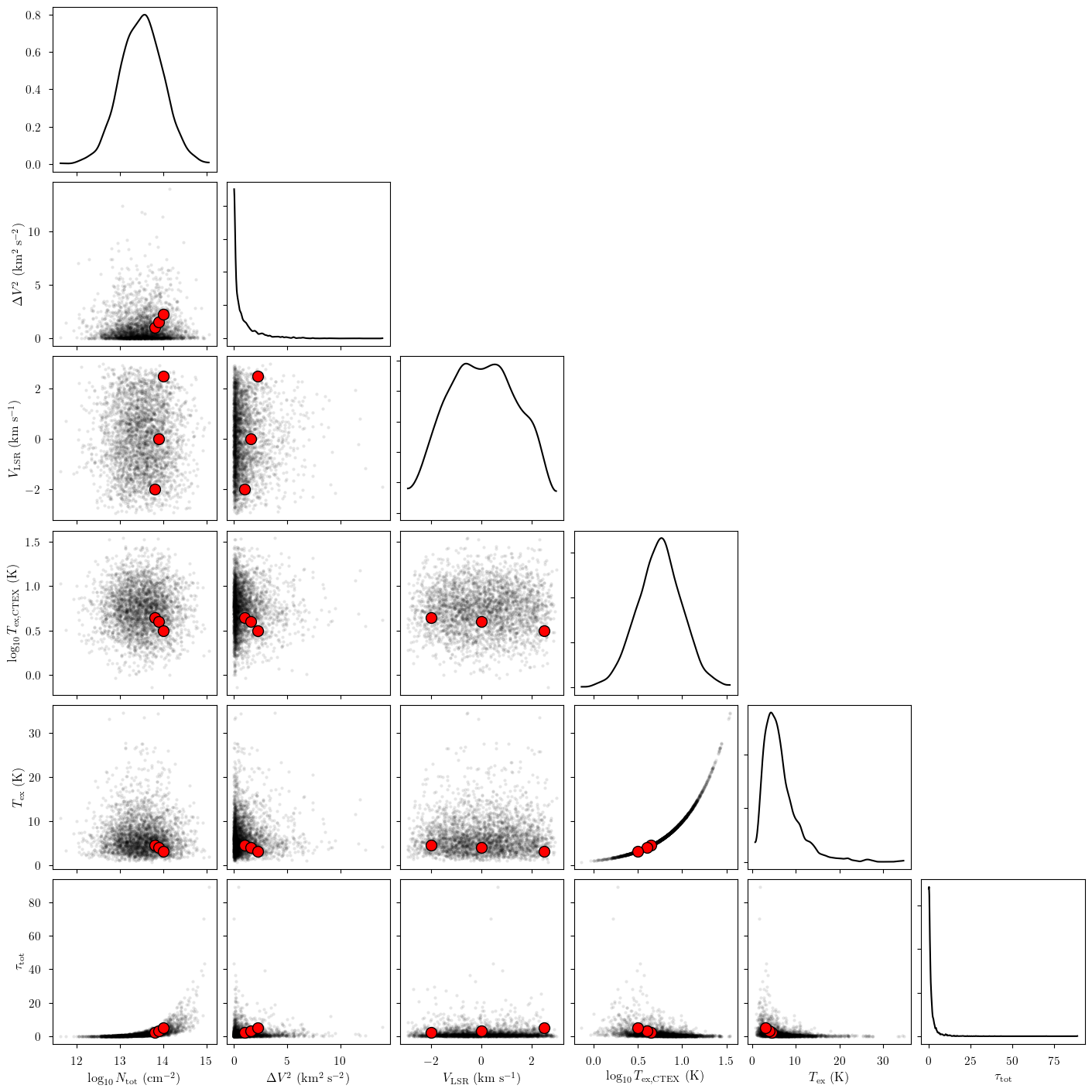
We can also check out our prior distributions impact the deterministic (derived) quantities in our model. The red points represent the simulation parameters.
[13]:
print(model.cloud_freeRVs)
print(model.cloud_deterministics)
['log10_Ntot_norm', 'fwhm2_norm', 'velocity_norm', 'log10_Tex_CTEX_norm']
['log10_Ntot', 'fwhm2', 'velocity', 'log10_Tex_CTEX', 'CTEX_weights', 'Tex', 'tau', 'tau_total', 'TR']
[14]:
from bayes_spec.plots import plot_pair

var_names = [
    param for param in model.cloud_deterministics + [p for p in model.cloud_freeRVs if "_norm" not in p]
    if not set(model.model.named_vars_to_dims[param]).intersection(set(["transition", "state"]))
]
print(var_names)
_ = plot_pair(
    prior.prior, # samples
    var_names, # var_names to plot
    combine_dims=["cloud"], # concatenate clouds
    labeller=model.labeller, # label manager
    kind="scatter", # plot type
    reference_values=sim_params, # truths
)
['log10_Ntot', 'fwhm2', 'velocity', 'log10_Tex_CTEX', 'Tex', 'tau_total']
Variational Inference
We can approximate the posterior distribution using variational inference.
[15]:
start = time.time()
model.fit(
    n = 1_000_000, # maximum number of VI iterations
    draws = 1_000, # number of posterior samples
    rel_tolerance = 0.005, # VI relative convergence threshold
    abs_tolerance = 0.005, # VI absolute convergence threshold
    learning_rate = 0.001, # VI learning rate
    start = {"velocity_norm": np.linspace(0.1, 0.9, model.n_clouds)},
)
end = time.time()
print(f"Runtime: {(end-start)/60.0:.2f} minutes")
Convergence achieved at 26300
Interrupted at 26,299 [2%]: Average Loss = -762.32
Adding log-likelihood to trace
Runtime: 3.99 minutes
[16]:
pm.summary(model.trace.posterior)
arviz - WARNING - Shape validation failed: input_shape: (1, 1000), minimum_shape: (chains=2, draws=4)
/home/twenger/miniforge3/envs/bayes_spec-dev/lib/python3.13/site-packages/arviz/stats/diagnostics.py:991: RuntimeWarning: invalid value encountered in scalar divide
  varsd = varvar / evar / 4
/home/twenger/miniforge3/envs/bayes_spec-dev/lib/python3.13/site-packages/arviz/stats/diagnostics.py:991: RuntimeWarning: invalid value encountered in scalar divide
  varsd = varvar / evar / 4
/home/twenger/miniforge3/envs/bayes_spec-dev/lib/python3.13/site-packages/arviz/stats/diagnostics.py:991: RuntimeWarning: invalid value encountered in scalar divide
  varsd = varvar / evar / 4
[16]:
| mean | sd | hdi_3% | hdi_97% | mcse_mean | mcse_sd | ess_bulk | ess_tail | r_hat | |
|---|---|---|---|---|---|---|---|---|---|
| baseline_12CN-1_norm[0] | 0.048 | 0.044 | -0.028 | 0.130 | 0.001 | 0.001 | 985.0 | 943.0 | NaN |
| baseline_12CN-2_norm[0] | 0.069 | 0.058 | -0.040 | 0.176 | 0.002 | 0.001 | 904.0 | 944.0 | NaN |
| log10_Ntot_norm[0] | 0.677 | 0.016 | 0.649 | 0.706 | 0.000 | 0.000 | 1061.0 | 981.0 | NaN |
| log10_Ntot_norm[1] | 0.749 | 0.018 | 0.716 | 0.783 | 0.001 | 0.000 | 742.0 | 923.0 | NaN |
| log10_Ntot_norm[2] | 0.947 | 0.042 | 0.866 | 1.024 | 0.001 | 0.001 | 946.0 | 982.0 | NaN |
| log10_Tex_CTEX_norm[0] | -0.467 | 0.009 | -0.482 | -0.449 | 0.000 | 0.000 | 957.0 | 876.0 | NaN |
| log10_Tex_CTEX_norm[1] | -0.579 | 0.009 | -0.596 | -0.562 | 0.000 | 0.000 | 858.0 | 905.0 | NaN |
| log10_Tex_CTEX_norm[2] | -0.993 | 0.009 | -1.010 | -0.978 | 0.000 | 0.000 | 788.0 | 891.0 | NaN |
| fwhm2_norm[0] | 0.986 | 0.043 | 0.904 | 1.061 | 0.001 | 0.001 | 1152.0 | 983.0 | NaN |
| fwhm2_norm[1] | 1.673 | 0.079 | 1.529 | 1.819 | 0.003 | 0.002 | 939.0 | 909.0 | NaN |
| fwhm2_norm[2] | 2.255 | 0.226 | 1.869 | 2.714 | 0.007 | 0.005 | 945.0 | 841.0 | NaN |
| velocity_norm[0] | 0.165 | 0.002 | 0.163 | 0.168 | 0.000 | 0.000 | 1082.0 | 1014.0 | NaN |
| velocity_norm[1] | 0.499 | 0.002 | 0.495 | 0.504 | 0.000 | 0.000 | 1032.0 | 901.0 | NaN |
| velocity_norm[2] | 0.918 | 0.006 | 0.908 | 0.928 | 0.000 | 0.000 | 971.0 | 808.0 | NaN |
| log10_Ntot[0] | 13.839 | 0.008 | 13.824 | 13.853 | 0.000 | 0.000 | 1061.0 | 981.0 | NaN |
| log10_Ntot[1] | 13.875 | 0.009 | 13.858 | 13.891 | 0.000 | 0.000 | 742.0 | 923.0 | NaN |
| log10_Ntot[2] | 13.974 | 0.021 | 13.933 | 14.012 | 0.001 | 0.000 | 946.0 | 982.0 | NaN |
| fwhm2[0] | 0.986 | 0.043 | 0.904 | 1.061 | 0.001 | 0.001 | 1152.0 | 983.0 | NaN |
| fwhm2[1] | 1.673 | 0.079 | 1.529 | 1.819 | 0.003 | 0.002 | 939.0 | 909.0 | NaN |
| fwhm2[2] | 2.255 | 0.226 | 1.869 | 2.714 | 0.007 | 0.005 | 945.0 | 841.0 | NaN |
| velocity[0] | -2.008 | 0.009 | -2.025 | -1.991 | 0.000 | 0.000 | 1082.0 | 1014.0 | NaN |
| velocity[1] | -0.004 | 0.014 | -0.028 | 0.022 | 0.000 | 0.000 | 1032.0 | 901.0 | NaN |
| velocity[2] | 2.505 | 0.033 | 2.448 | 2.569 | 0.001 | 0.001 | 971.0 | 808.0 | NaN |
| log10_Tex_CTEX[0] | 0.633 | 0.002 | 0.629 | 0.638 | 0.000 | 0.000 | 957.0 | 876.0 | NaN |
| log10_Tex_CTEX[1] | 0.605 | 0.002 | 0.601 | 0.610 | 0.000 | 0.000 | 858.0 | 905.0 | NaN |
| log10_Tex_CTEX[2] | 0.502 | 0.002 | 0.497 | 0.506 | 0.000 | 0.000 | 788.0 | 891.0 | NaN |
| CTEX_weights[0, 0 0 1 1 -- --] | 2.000 | 0.000 | 2.000 | 2.000 | 0.000 | 0.000 | 957.0 | 876.0 | NaN |
| CTEX_weights[0, 0 0 1 2 -- --] | 4.000 | 0.000 | 4.000 | 4.000 | 0.000 | NaN | 1000.0 | 1000.0 | NaN |
| CTEX_weights[0, 1 0 1 1 -- --] | 0.566 | 0.004 | 0.559 | 0.572 | 0.000 | 0.000 | 957.0 | 876.0 | NaN |
| CTEX_weights[0, 1 0 1 2 -- --] | 1.131 | 0.007 | 1.117 | 1.144 | 0.000 | 0.000 | 957.0 | 876.0 | NaN |
| CTEX_weights[0, 1 0 2 1 -- --] | 0.563 | 0.004 | 0.556 | 0.570 | 0.000 | 0.000 | 957.0 | 876.0 | NaN |
| CTEX_weights[0, 1 0 2 2 -- --] | 1.127 | 0.007 | 1.113 | 1.140 | 0.000 | 0.000 | 957.0 | 876.0 | NaN |
| CTEX_weights[0, 1 0 2 3 -- --] | 1.690 | 0.011 | 1.669 | 1.710 | 0.000 | 0.000 | 957.0 | 876.0 | NaN |
| CTEX_weights[1, 0 0 1 1 -- --] | 2.000 | 0.000 | 1.999 | 2.000 | 0.000 | 0.000 | 858.0 | 905.0 | NaN |
| CTEX_weights[1, 0 0 1 2 -- --] | 4.000 | 0.000 | 4.000 | 4.000 | 0.000 | NaN | 1000.0 | 1000.0 | NaN |
| CTEX_weights[1, 1 0 1 1 -- --] | 0.520 | 0.004 | 0.513 | 0.527 | 0.000 | 0.000 | 858.0 | 905.0 | NaN |
| CTEX_weights[1, 1 0 1 2 -- --] | 1.039 | 0.007 | 1.025 | 1.053 | 0.000 | 0.000 | 858.0 | 905.0 | NaN |
| CTEX_weights[1, 1 0 2 1 -- --] | 0.517 | 0.004 | 0.511 | 0.524 | 0.000 | 0.000 | 858.0 | 905.0 | NaN |
| CTEX_weights[1, 1 0 2 2 -- --] | 1.035 | 0.007 | 1.021 | 1.049 | 0.000 | 0.000 | 858.0 | 905.0 | NaN |
| CTEX_weights[1, 1 0 2 3 -- --] | 1.553 | 0.011 | 1.532 | 1.574 | 0.000 | 0.000 | 858.0 | 905.0 | NaN |
| CTEX_weights[2, 0 0 1 1 -- --] | 1.999 | 0.000 | 1.999 | 1.999 | 0.000 | 0.000 | 788.0 | 891.0 | NaN |
| CTEX_weights[2, 0 0 1 2 -- --] | 4.000 | 0.000 | 4.000 | 4.000 | 0.000 | NaN | 1000.0 | 1000.0 | NaN |
| CTEX_weights[2, 1 0 1 1 -- --] | 0.362 | 0.003 | 0.356 | 0.367 | 0.000 | 0.000 | 788.0 | 891.0 | NaN |
| CTEX_weights[2, 1 0 1 2 -- --] | 0.723 | 0.006 | 0.711 | 0.734 | 0.000 | 0.000 | 788.0 | 891.0 | NaN |
| CTEX_weights[2, 1 0 2 1 -- --] | 0.360 | 0.003 | 0.354 | 0.365 | 0.000 | 0.000 | 788.0 | 891.0 | NaN |
| CTEX_weights[2, 1 0 2 2 -- --] | 0.719 | 0.006 | 0.707 | 0.730 | 0.000 | 0.000 | 788.0 | 891.0 | NaN |
| CTEX_weights[2, 1 0 2 3 -- --] | 1.079 | 0.009 | 1.061 | 1.095 | 0.000 | 0.000 | 788.0 | 891.0 | NaN |
| Tex[0] | 4.299 | 0.023 | 4.257 | 4.340 | 0.001 | 0.000 | 957.0 | 876.0 | NaN |
| Tex[1] | 4.029 | 0.021 | 3.990 | 4.070 | 0.001 | 0.000 | 858.0 | 905.0 | NaN |
| Tex[2] | 3.175 | 0.016 | 3.144 | 3.203 | 0.001 | 0.000 | 788.0 | 891.0 | NaN |
| tau[113123.3701, 0] | 0.031 | 0.001 | 0.030 | 0.032 | 0.000 | 0.000 | 1053.0 | 841.0 | NaN |
| tau[113123.3701, 1] | 0.036 | 0.001 | 0.035 | 0.038 | 0.000 | 0.000 | 725.0 | 1066.0 | NaN |
| tau[113123.3701, 2] | 0.058 | 0.003 | 0.053 | 0.063 | 0.000 | 0.000 | 945.0 | 983.0 | NaN |
| tau[113144.1573, 0] | 0.255 | 0.005 | 0.247 | 0.264 | 0.000 | 0.000 | 1053.0 | 841.0 | NaN |
| tau[113144.1573, 1] | 0.297 | 0.006 | 0.286 | 0.310 | 0.000 | 0.000 | 725.0 | 1066.0 | NaN |
| tau[113144.1573, 2] | 0.477 | 0.023 | 0.431 | 0.519 | 0.001 | 0.001 | 945.0 | 983.0 | NaN |
| tau[113170.4915, 0] | 0.249 | 0.005 | 0.241 | 0.257 | 0.000 | 0.000 | 1053.0 | 841.0 | NaN |
| tau[113170.4915, 1] | 0.290 | 0.006 | 0.280 | 0.302 | 0.000 | 0.000 | 725.0 | 1066.0 | NaN |
| tau[113170.4915, 2] | 0.466 | 0.023 | 0.421 | 0.506 | 0.001 | 0.001 | 945.0 | 983.0 | NaN |
| tau[113191.2787, 0] | 0.324 | 0.006 | 0.313 | 0.334 | 0.000 | 0.000 | 1053.0 | 841.0 | NaN |
| tau[113191.2787, 1] | 0.377 | 0.008 | 0.363 | 0.393 | 0.000 | 0.000 | 725.0 | 1066.0 | NaN |
| tau[113191.2787, 2] | 0.606 | 0.030 | 0.547 | 0.658 | 0.001 | 0.001 | 945.0 | 983.0 | NaN |
| tau[113488.1202, 0] | 0.325 | 0.006 | 0.314 | 0.336 | 0.000 | 0.000 | 1053.0 | 841.0 | NaN |
| tau[113488.1202, 1] | 0.378 | 0.008 | 0.365 | 0.394 | 0.000 | 0.000 | 725.0 | 1066.0 | NaN |
| tau[113488.1202, 2] | 0.608 | 0.030 | 0.549 | 0.660 | 0.001 | 0.001 | 945.0 | 983.0 | NaN |
| tau[113490.9702, 0] | 0.863 | 0.016 | 0.834 | 0.891 | 0.000 | 0.000 | 1053.0 | 841.0 | NaN |
| tau[113490.9702, 1] | 1.005 | 0.022 | 0.968 | 1.047 | 0.001 | 0.001 | 725.0 | 1066.0 | NaN |
| tau[113490.9702, 2] | 1.614 | 0.079 | 1.459 | 1.753 | 0.003 | 0.002 | 945.0 | 983.0 | NaN |
| tau[113499.6443, 0] | 0.256 | 0.005 | 0.248 | 0.265 | 0.000 | 0.000 | 1053.0 | 841.0 | NaN |
| tau[113499.6443, 1] | 0.299 | 0.006 | 0.288 | 0.311 | 0.000 | 0.000 | 725.0 | 1066.0 | NaN |
| tau[113499.6443, 2] | 0.479 | 0.023 | 0.433 | 0.521 | 0.001 | 0.001 | 945.0 | 983.0 | NaN |
| tau[113508.9074, 0] | 0.250 | 0.005 | 0.242 | 0.259 | 0.000 | 0.000 | 1053.0 | 841.0 | NaN |
| tau[113508.9074, 1] | 0.292 | 0.006 | 0.281 | 0.304 | 0.000 | 0.000 | 725.0 | 1066.0 | NaN |
| tau[113508.9074, 2] | 0.468 | 0.023 | 0.423 | 0.509 | 0.001 | 0.001 | 945.0 | 983.0 | NaN |
| tau[113520.4315, 0] | 0.031 | 0.001 | 0.030 | 0.032 | 0.000 | 0.000 | 1053.0 | 841.0 | NaN |
| tau[113520.4315, 1] | 0.037 | 0.001 | 0.035 | 0.038 | 0.000 | 0.000 | 725.0 | 1066.0 | NaN |
| tau[113520.4315, 2] | 0.059 | 0.003 | 0.053 | 0.064 | 0.000 | 0.000 | 945.0 | 983.0 | NaN |
| tau_total[0] | 2.586 | 0.048 | 2.498 | 2.670 | 0.001 | 0.001 | 1053.0 | 841.0 | NaN |
| tau_total[1] | 3.011 | 0.064 | 2.901 | 3.136 | 0.002 | 0.002 | 725.0 | 1066.0 | NaN |
| tau_total[2] | 4.835 | 0.237 | 4.370 | 5.252 | 0.008 | 0.005 | 945.0 | 983.0 | NaN |
| TR[113123.3701, 0] | 2.141 | 0.020 | 2.105 | 2.177 | 0.001 | 0.000 | 957.0 | 876.0 | NaN |
| TR[113123.3701, 1] | 1.907 | 0.018 | 1.873 | 1.941 | 0.001 | 0.000 | 858.0 | 905.0 | NaN |
| TR[113123.3701, 2] | 1.199 | 0.012 | 1.174 | 1.221 | 0.000 | 0.000 | 788.0 | 891.0 | NaN |
| TR[113144.1573, 0] | 2.141 | 0.020 | 2.104 | 2.177 | 0.001 | 0.000 | 957.0 | 876.0 | NaN |
| TR[113144.1573, 1] | 1.907 | 0.018 | 1.873 | 1.941 | 0.001 | 0.000 | 858.0 | 905.0 | NaN |
| TR[113144.1573, 2] | 1.199 | 0.012 | 1.174 | 1.221 | 0.000 | 0.000 | 788.0 | 891.0 | NaN |
| TR[113170.4915, 0] | 2.141 | 0.020 | 2.104 | 2.176 | 0.001 | 0.000 | 957.0 | 876.0 | NaN |
| TR[113170.4915, 1] | 1.906 | 0.018 | 1.872 | 1.941 | 0.001 | 0.000 | 858.0 | 905.0 | NaN |
| TR[113170.4915, 2] | 1.198 | 0.012 | 1.174 | 1.220 | 0.000 | 0.000 | 788.0 | 891.0 | NaN |
| TR[113191.2787, 0] | 2.140 | 0.020 | 2.104 | 2.176 | 0.001 | 0.000 | 957.0 | 876.0 | NaN |
| TR[113191.2787, 1] | 1.906 | 0.018 | 1.872 | 1.941 | 0.001 | 0.000 | 858.0 | 905.0 | NaN |
| TR[113191.2787, 2] | 1.198 | 0.012 | 1.174 | 1.220 | 0.000 | 0.000 | 788.0 | 891.0 | NaN |
| TR[113488.1202, 0] | 2.136 | 0.020 | 2.099 | 2.172 | 0.001 | 0.000 | 957.0 | 876.0 | NaN |
| TR[113488.1202, 1] | 1.902 | 0.018 | 1.868 | 1.936 | 0.001 | 0.000 | 858.0 | 905.0 | NaN |
| TR[113488.1202, 2] | 1.195 | 0.012 | 1.170 | 1.217 | 0.000 | 0.000 | 788.0 | 891.0 | NaN |
| TR[113490.9702, 0] | 2.136 | 0.020 | 2.099 | 2.172 | 0.001 | 0.000 | 957.0 | 876.0 | NaN |
| TR[113490.9702, 1] | 1.902 | 0.018 | 1.868 | 1.936 | 0.001 | 0.000 | 858.0 | 905.0 | NaN |
| TR[113490.9702, 2] | 1.195 | 0.012 | 1.170 | 1.217 | 0.000 | 0.000 | 788.0 | 891.0 | NaN |
| TR[113499.6443, 0] | 2.136 | 0.020 | 2.099 | 2.172 | 0.001 | 0.000 | 957.0 | 876.0 | NaN |
| TR[113499.6443, 1] | 1.902 | 0.018 | 1.868 | 1.936 | 0.001 | 0.000 | 858.0 | 905.0 | NaN |
| TR[113499.6443, 2] | 1.195 | 0.012 | 1.170 | 1.216 | 0.000 | 0.000 | 788.0 | 891.0 | NaN |
| TR[113508.9074, 0] | 2.136 | 0.020 | 2.099 | 2.171 | 0.001 | 0.000 | 957.0 | 876.0 | NaN |
| TR[113508.9074, 1] | 1.901 | 0.018 | 1.868 | 1.936 | 0.001 | 0.000 | 858.0 | 905.0 | NaN |
| TR[113508.9074, 2] | 1.195 | 0.012 | 1.170 | 1.216 | 0.000 | 0.000 | 788.0 | 891.0 | NaN |
| TR[113520.4315, 0] | 2.136 | 0.020 | 2.099 | 2.171 | 0.001 | 0.000 | 957.0 | 876.0 | NaN |
| TR[113520.4315, 1] | 1.901 | 0.018 | 1.867 | 1.936 | 0.001 | 0.000 | 858.0 | 905.0 | NaN |
| TR[113520.4315, 2] | 1.194 | 0.012 | 1.170 | 1.216 | 0.000 | 0.000 | 788.0 | 891.0 | NaN |
[17]:
posterior = model.sample_posterior_predictive(
    thin=100, # keep one in {thin} posterior samples
)
_ = plot_predictive(model.data, posterior.posterior_predictive)
Sampling: [12CN-1, 12CN-2]
Posterior Sampling: MCMC
We can sample from the posterior distribution using MCMC.
[18]:
start = time.time()
model.sample(
    init="advi+adapt_diag",  # initialization strategy
    tune=1000,  # tuning samples
    draws=1000,  # posterior samples
    chains=8,  # number of independent chains
    cores=8,  # number of parallel chains
    init_kwargs={
        "rel_tolerance": 0.005,
        "abs_tolerance": 0.005,
        "learning_rate": 0.001,
        "start": {"velocity_norm": np.linspace(0.1, 0.9, model.n_clouds)},
    },  # VI initialization arguments
    nuts_kwargs={"target_accept": 0.8},  # NUTS arguments
)
end = time.time()
print(f"Runtime: {(end-start)/60.0:.2f} minutes")
Initializing NUTS using custom advi+adapt_diag strategy
Convergence achieved at 26300
Interrupted at 26,299 [2%]: Average Loss = -762.32
Multiprocess sampling (8 chains in 8 jobs)
NUTS: [baseline_12CN-1_norm, baseline_12CN-2_norm, log10_Ntot_norm, fwhm2_norm, velocity_norm, log10_Tex_CTEX_norm]
Sampling 8 chains for 1_000 tune and 1_000 draw iterations (8_000 + 8_000 draws total) took 69 seconds.
Adding log-likelihood to trace
Runtime: 5.53 minutes
[19]:
model.solve(
    init_params="random_from_data", # GMM initialization strategy
    n_init=10, # number of GMM initilizations
    max_iter=1_000, # maximum number of GMM iterations
    kl_div_threshold=0.1, # covergence threshold
)
GMM converged to unique solution
Check that the effective sample sizes are large and the covergence statistic r_hat is close to 1! If not, you may have to increase the number of tuning steps (tune=2000) or the NUTS acceptance rate (target_accept=0.9).
[20]:
print("solutions:", model.solutions)
az.summary(model.trace.solution_0)
# this also works: az.summary(model.trace.solution_0)
solutions: [0]
/home/twenger/miniforge3/envs/bayes_spec-dev/lib/python3.13/site-packages/arviz/stats/diagnostics.py:596: RuntimeWarning: invalid value encountered in scalar divide
  (between_chain_variance / within_chain_variance + num_samples - 1) / (num_samples)
/home/twenger/miniforge3/envs/bayes_spec-dev/lib/python3.13/site-packages/arviz/stats/diagnostics.py:991: RuntimeWarning: invalid value encountered in scalar divide
  varsd = varvar / evar / 4
[20]:
| mean | sd | hdi_3% | hdi_97% | mcse_mean | mcse_sd | ess_bulk | ess_tail | r_hat | |
|---|---|---|---|---|---|---|---|---|---|
| baseline_12CN-1_norm[0] | 0.046 | 0.043 | -0.031 | 0.130 | 0.000 | 0.001 | 12969.0 | 5767.0 | 1.0 |
| baseline_12CN-2_norm[0] | 0.069 | 0.062 | -0.050 | 0.180 | 0.001 | 0.001 | 13207.0 | 5704.0 | 1.0 |
| log10_Ntot_norm[0] | 0.675 | 0.044 | 0.589 | 0.752 | 0.001 | 0.000 | 6158.0 | 6125.0 | 1.0 |
| log10_Ntot_norm[1] | 0.743 | 0.055 | 0.640 | 0.849 | 0.001 | 0.001 | 6912.0 | 4804.0 | 1.0 |
| log10_Ntot_norm[2] | 0.942 | 0.128 | 0.701 | 1.183 | 0.002 | 0.001 | 6127.0 | 5162.0 | 1.0 |
| log10_Tex_CTEX_norm[0] | -0.463 | 0.027 | -0.512 | -0.415 | 0.000 | 0.000 | 6182.0 | 6267.0 | 1.0 |
| log10_Tex_CTEX_norm[1] | -0.577 | 0.030 | -0.635 | -0.522 | 0.000 | 0.000 | 6909.0 | 5201.0 | 1.0 |
| log10_Tex_CTEX_norm[2] | -0.989 | 0.026 | -1.035 | -0.940 | 0.000 | 0.000 | 6071.0 | 4938.0 | 1.0 |
| fwhm2_norm[0] | 0.988 | 0.051 | 0.894 | 1.085 | 0.001 | 0.001 | 8883.0 | 6932.0 | 1.0 |
| fwhm2_norm[1] | 1.666 | 0.112 | 1.464 | 1.881 | 0.001 | 0.001 | 7040.0 | 6042.0 | 1.0 |
| fwhm2_norm[2] | 2.285 | 0.273 | 1.781 | 2.799 | 0.003 | 0.003 | 9457.0 | 6409.0 | 1.0 |
| velocity_norm[0] | 0.165 | 0.002 | 0.162 | 0.168 | 0.000 | 0.000 | 8846.0 | 6461.0 | 1.0 |
| velocity_norm[1] | 0.500 | 0.003 | 0.494 | 0.504 | 0.000 | 0.000 | 9664.0 | 6577.0 | 1.0 |
| velocity_norm[2] | 0.918 | 0.007 | 0.905 | 0.930 | 0.000 | 0.000 | 9963.0 | 6209.0 | 1.0 |
| log10_Ntot[0] | 13.837 | 0.022 | 13.794 | 13.876 | 0.000 | 0.000 | 6158.0 | 6125.0 | 1.0 |
| log10_Ntot[1] | 13.872 | 0.028 | 13.820 | 13.925 | 0.000 | 0.000 | 6912.0 | 4804.0 | 1.0 |
| log10_Ntot[2] | 13.971 | 0.064 | 13.851 | 14.091 | 0.001 | 0.001 | 6127.0 | 5162.0 | 1.0 |
| fwhm2[0] | 0.988 | 0.051 | 0.894 | 1.085 | 0.001 | 0.001 | 8883.0 | 6932.0 | 1.0 |
| fwhm2[1] | 1.666 | 0.112 | 1.464 | 1.881 | 0.001 | 0.001 | 7040.0 | 6042.0 | 1.0 |
| fwhm2[2] | 2.285 | 0.273 | 1.781 | 2.799 | 0.003 | 0.003 | 9457.0 | 6409.0 | 1.0 |
| velocity[0] | -2.010 | 0.011 | -2.029 | -1.990 | 0.000 | 0.000 | 8846.0 | 6461.0 | 1.0 |
| velocity[1] | -0.003 | 0.016 | -0.033 | 0.025 | 0.000 | 0.000 | 9664.0 | 6577.0 | 1.0 |
| velocity[2] | 2.506 | 0.039 | 2.432 | 2.578 | 0.000 | 0.000 | 9963.0 | 6209.0 | 1.0 |
| log10_Tex_CTEX[0] | 0.634 | 0.007 | 0.622 | 0.646 | 0.000 | 0.000 | 6182.0 | 6267.0 | 1.0 |
| log10_Tex_CTEX[1] | 0.606 | 0.007 | 0.591 | 0.619 | 0.000 | 0.000 | 6909.0 | 5201.0 | 1.0 |
| log10_Tex_CTEX[2] | 0.503 | 0.006 | 0.491 | 0.515 | 0.000 | 0.000 | 6071.0 | 4938.0 | 1.0 |
| CTEX_weights[0, 0 0 1 1 -- --] | 2.000 | 0.000 | 2.000 | 2.000 | 0.000 | 0.000 | 6182.0 | 6267.0 | 1.0 |
| CTEX_weights[0, 0 0 1 2 -- --] | 4.000 | 0.000 | 4.000 | 4.000 | 0.000 | NaN | 8000.0 | 8000.0 | NaN |
| CTEX_weights[0, 1 0 1 1 -- --] | 0.567 | 0.011 | 0.547 | 0.587 | 0.000 | 0.000 | 6182.0 | 6267.0 | 1.0 |
| CTEX_weights[0, 1 0 1 2 -- --] | 1.133 | 0.022 | 1.093 | 1.173 | 0.000 | 0.000 | 6182.0 | 6267.0 | 1.0 |
| CTEX_weights[0, 1 0 2 1 -- --] | 0.565 | 0.011 | 0.544 | 0.585 | 0.000 | 0.000 | 6182.0 | 6267.0 | 1.0 |
| CTEX_weights[0, 1 0 2 2 -- --] | 1.129 | 0.022 | 1.089 | 1.169 | 0.000 | 0.000 | 6182.0 | 6267.0 | 1.0 |
| CTEX_weights[0, 1 0 2 3 -- --] | 1.694 | 0.033 | 1.634 | 1.754 | 0.000 | 0.000 | 6182.0 | 6267.0 | 1.0 |
| CTEX_weights[1, 0 0 1 1 -- --] | 2.000 | 0.000 | 1.999 | 2.000 | 0.000 | 0.000 | 6909.0 | 5201.0 | 1.0 |
| CTEX_weights[1, 0 0 1 2 -- --] | 4.000 | 0.000 | 4.000 | 4.000 | 0.000 | NaN | 8000.0 | 8000.0 | NaN |
| CTEX_weights[1, 1 0 1 1 -- --] | 0.521 | 0.012 | 0.497 | 0.543 | 0.000 | 0.000 | 6909.0 | 5201.0 | 1.0 |
| CTEX_weights[1, 1 0 1 2 -- --] | 1.041 | 0.024 | 0.994 | 1.085 | 0.000 | 0.000 | 6909.0 | 5201.0 | 1.0 |
| CTEX_weights[1, 1 0 2 1 -- --] | 0.518 | 0.012 | 0.495 | 0.540 | 0.000 | 0.000 | 6909.0 | 5201.0 | 1.0 |
| CTEX_weights[1, 1 0 2 2 -- --] | 1.037 | 0.024 | 0.990 | 1.081 | 0.000 | 0.000 | 6909.0 | 5201.0 | 1.0 |
| CTEX_weights[1, 1 0 2 3 -- --] | 1.555 | 0.036 | 1.486 | 1.622 | 0.000 | 0.000 | 6909.0 | 5201.0 | 1.0 |
| CTEX_weights[2, 0 0 1 1 -- --] | 1.999 | 0.000 | 1.999 | 1.999 | 0.000 | 0.000 | 6071.0 | 4938.0 | 1.0 |
| CTEX_weights[2, 0 0 1 2 -- --] | 4.000 | 0.000 | 4.000 | 4.000 | 0.000 | NaN | 8000.0 | 8000.0 | NaN |
| CTEX_weights[2, 1 0 1 1 -- --] | 0.363 | 0.009 | 0.346 | 0.380 | 0.000 | 0.000 | 6071.0 | 4938.0 | 1.0 |
| CTEX_weights[2, 1 0 1 2 -- --] | 0.725 | 0.018 | 0.692 | 0.760 | 0.000 | 0.000 | 6071.0 | 4938.0 | 1.0 |
| CTEX_weights[2, 1 0 2 1 -- --] | 0.361 | 0.009 | 0.344 | 0.378 | 0.000 | 0.000 | 6071.0 | 4938.0 | 1.0 |
| CTEX_weights[2, 1 0 2 2 -- --] | 0.722 | 0.018 | 0.688 | 0.756 | 0.000 | 0.000 | 6071.0 | 4938.0 | 1.0 |
| CTEX_weights[2, 1 0 2 3 -- --] | 1.083 | 0.028 | 1.033 | 1.135 | 0.000 | 0.000 | 6071.0 | 4938.0 | 1.0 |
| Tex[0] | 4.307 | 0.066 | 4.187 | 4.430 | 0.001 | 0.001 | 6182.0 | 6267.0 | 1.0 |
| Tex[1] | 4.035 | 0.069 | 3.902 | 4.163 | 0.001 | 0.001 | 6909.0 | 5201.0 | 1.0 |
| Tex[2] | 3.182 | 0.047 | 3.095 | 3.271 | 0.001 | 0.001 | 6071.0 | 4938.0 | 1.0 |
| tau[113123.3701, 0] | 0.031 | 0.002 | 0.027 | 0.035 | 0.000 | 0.000 | 6124.0 | 5938.0 | 1.0 |
| tau[113123.3701, 1] | 0.036 | 0.003 | 0.031 | 0.042 | 0.000 | 0.000 | 6884.0 | 4877.0 | 1.0 |
| tau[113123.3701, 2] | 0.059 | 0.009 | 0.041 | 0.076 | 0.000 | 0.000 | 6106.0 | 4895.0 | 1.0 |
| tau[113144.1573, 0] | 0.255 | 0.017 | 0.224 | 0.286 | 0.000 | 0.000 | 6124.0 | 5938.0 | 1.0 |
| tau[113144.1573, 1] | 0.296 | 0.024 | 0.250 | 0.340 | 0.000 | 0.000 | 6884.0 | 4877.0 | 1.0 |
| tau[113144.1573, 2] | 0.479 | 0.077 | 0.338 | 0.623 | 0.001 | 0.001 | 6106.0 | 4895.0 | 1.0 |
| tau[113170.4915, 0] | 0.249 | 0.016 | 0.218 | 0.279 | 0.000 | 0.000 | 6124.0 | 5938.0 | 1.0 |
| tau[113170.4915, 1] | 0.289 | 0.023 | 0.244 | 0.332 | 0.000 | 0.000 | 6884.0 | 4877.0 | 1.0 |
| tau[113170.4915, 2] | 0.468 | 0.075 | 0.330 | 0.609 | 0.001 | 0.001 | 6106.0 | 4895.0 | 1.0 |
| tau[113191.2787, 0] | 0.323 | 0.021 | 0.284 | 0.362 | 0.000 | 0.000 | 6124.0 | 5938.0 | 1.0 |
| tau[113191.2787, 1] | 0.375 | 0.030 | 0.317 | 0.432 | 0.000 | 0.000 | 6884.0 | 4877.0 | 1.0 |
| tau[113191.2787, 2] | 0.608 | 0.098 | 0.429 | 0.791 | 0.001 | 0.001 | 6106.0 | 4895.0 | 1.0 |
| tau[113488.1202, 0] | 0.324 | 0.021 | 0.285 | 0.364 | 0.000 | 0.000 | 6124.0 | 5938.0 | 1.0 |
| tau[113488.1202, 1] | 0.377 | 0.030 | 0.318 | 0.433 | 0.000 | 0.000 | 6884.0 | 4877.0 | 1.0 |
| tau[113488.1202, 2] | 0.610 | 0.098 | 0.430 | 0.793 | 0.001 | 0.001 | 6106.0 | 4895.0 | 1.0 |
| tau[113490.9702, 0] | 0.861 | 0.057 | 0.756 | 0.966 | 0.001 | 0.001 | 6124.0 | 5938.0 | 1.0 |
| tau[113490.9702, 1] | 1.000 | 0.081 | 0.845 | 1.151 | 0.001 | 0.001 | 6884.0 | 4877.0 | 1.0 |
| tau[113490.9702, 2] | 1.620 | 0.260 | 1.143 | 2.107 | 0.003 | 0.003 | 6106.0 | 4895.0 | 1.0 |
| tau[113499.6443, 0] | 0.256 | 0.017 | 0.225 | 0.287 | 0.000 | 0.000 | 6124.0 | 5938.0 | 1.0 |
| tau[113499.6443, 1] | 0.297 | 0.024 | 0.251 | 0.342 | 0.000 | 0.000 | 6884.0 | 4877.0 | 1.0 |
| tau[113499.6443, 2] | 0.481 | 0.077 | 0.339 | 0.626 | 0.001 | 0.001 | 6106.0 | 4895.0 | 1.0 |
| tau[113508.9074, 0] | 0.250 | 0.016 | 0.219 | 0.280 | 0.000 | 0.000 | 6124.0 | 5938.0 | 1.0 |
| tau[113508.9074, 1] | 0.290 | 0.023 | 0.245 | 0.334 | 0.000 | 0.000 | 6884.0 | 4877.0 | 1.0 |
| tau[113508.9074, 2] | 0.470 | 0.075 | 0.332 | 0.611 | 0.001 | 0.001 | 6106.0 | 4895.0 | 1.0 |
| tau[113520.4315, 0] | 0.031 | 0.002 | 0.027 | 0.035 | 0.000 | 0.000 | 6124.0 | 5938.0 | 1.0 |
| tau[113520.4315, 1] | 0.036 | 0.003 | 0.031 | 0.042 | 0.000 | 0.000 | 6884.0 | 4877.0 | 1.0 |
| tau[113520.4315, 2] | 0.059 | 0.009 | 0.041 | 0.077 | 0.000 | 0.000 | 6106.0 | 4895.0 | 1.0 |
| tau_total[0] | 2.578 | 0.169 | 2.265 | 2.894 | 0.002 | 0.002 | 6124.0 | 5938.0 | 1.0 |
| tau_total[1] | 2.997 | 0.242 | 2.532 | 3.448 | 0.003 | 0.003 | 6884.0 | 4877.0 | 1.0 |
| tau_total[2] | 4.852 | 0.779 | 3.424 | 6.314 | 0.010 | 0.009 | 6106.0 | 4895.0 | 1.0 |
| TR[113123.3701, 0] | 2.149 | 0.058 | 2.043 | 2.256 | 0.001 | 0.001 | 6182.0 | 6267.0 | 1.0 |
| TR[113123.3701, 1] | 1.912 | 0.060 | 1.798 | 2.023 | 0.001 | 0.001 | 6909.0 | 5201.0 | 1.0 |
| TR[113123.3701, 2] | 1.204 | 0.037 | 1.136 | 1.275 | 0.000 | 0.000 | 6071.0 | 4938.0 | 1.0 |
| TR[113144.1573, 0] | 2.148 | 0.058 | 2.043 | 2.256 | 0.001 | 0.001 | 6182.0 | 6267.0 | 1.0 |
| TR[113144.1573, 1] | 1.911 | 0.060 | 1.797 | 2.022 | 0.001 | 0.001 | 6909.0 | 5201.0 | 1.0 |
| TR[113144.1573, 2] | 1.204 | 0.037 | 1.136 | 1.274 | 0.000 | 0.000 | 6071.0 | 4938.0 | 1.0 |
| TR[113170.4915, 0] | 2.148 | 0.058 | 2.042 | 2.255 | 0.001 | 0.001 | 6182.0 | 6267.0 | 1.0 |
| TR[113170.4915, 1] | 1.911 | 0.060 | 1.797 | 2.022 | 0.001 | 0.001 | 6909.0 | 5201.0 | 1.0 |
| TR[113170.4915, 2] | 1.204 | 0.037 | 1.136 | 1.274 | 0.000 | 0.000 | 6071.0 | 4938.0 | 1.0 |
| TR[113191.2787, 0] | 2.148 | 0.058 | 2.042 | 2.255 | 0.001 | 0.001 | 6182.0 | 6267.0 | 1.0 |
| TR[113191.2787, 1] | 1.911 | 0.060 | 1.797 | 2.022 | 0.001 | 0.001 | 6909.0 | 5201.0 | 1.0 |
| TR[113191.2787, 2] | 1.204 | 0.037 | 1.136 | 1.274 | 0.000 | 0.000 | 6071.0 | 4938.0 | 1.0 |
| TR[113488.1202, 0] | 2.143 | 0.058 | 2.038 | 2.251 | 0.001 | 0.001 | 6182.0 | 6267.0 | 1.0 |
| TR[113488.1202, 1] | 1.907 | 0.060 | 1.793 | 2.017 | 0.001 | 0.001 | 6909.0 | 5201.0 | 1.0 |
| TR[113488.1202, 2] | 1.200 | 0.037 | 1.132 | 1.270 | 0.000 | 0.000 | 6071.0 | 4938.0 | 1.0 |
| TR[113490.9702, 0] | 2.143 | 0.058 | 2.038 | 2.251 | 0.001 | 0.001 | 6182.0 | 6267.0 | 1.0 |
| TR[113490.9702, 1] | 1.907 | 0.060 | 1.793 | 2.017 | 0.001 | 0.001 | 6909.0 | 5201.0 | 1.0 |
| TR[113490.9702, 2] | 1.200 | 0.037 | 1.132 | 1.270 | 0.000 | 0.000 | 6071.0 | 4938.0 | 1.0 |
| TR[113499.6443, 0] | 2.143 | 0.058 | 2.038 | 2.251 | 0.001 | 0.001 | 6182.0 | 6267.0 | 1.0 |
| TR[113499.6443, 1] | 1.906 | 0.060 | 1.792 | 2.017 | 0.001 | 0.001 | 6909.0 | 5201.0 | 1.0 |
| TR[113499.6443, 2] | 1.200 | 0.037 | 1.132 | 1.270 | 0.000 | 0.000 | 6071.0 | 4938.0 | 1.0 |
| TR[113508.9074, 0] | 2.143 | 0.058 | 2.038 | 2.251 | 0.001 | 0.001 | 6182.0 | 6267.0 | 1.0 |
| TR[113508.9074, 1] | 1.906 | 0.060 | 1.792 | 2.017 | 0.001 | 0.001 | 6909.0 | 5201.0 | 1.0 |
| TR[113508.9074, 2] | 1.200 | 0.037 | 1.132 | 1.270 | 0.000 | 0.000 | 6071.0 | 4938.0 | 1.0 |
| TR[113520.4315, 0] | 2.143 | 0.058 | 2.037 | 2.250 | 0.001 | 0.001 | 6182.0 | 6267.0 | 1.0 |
| TR[113520.4315, 1] | 1.906 | 0.060 | 1.792 | 2.017 | 0.001 | 0.001 | 6909.0 | 5201.0 | 1.0 |
| TR[113520.4315, 2] | 1.200 | 0.037 | 1.132 | 1.270 | 0.000 | 0.000 | 6071.0 | 4938.0 | 1.0 |
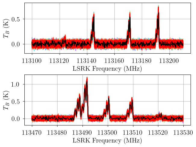
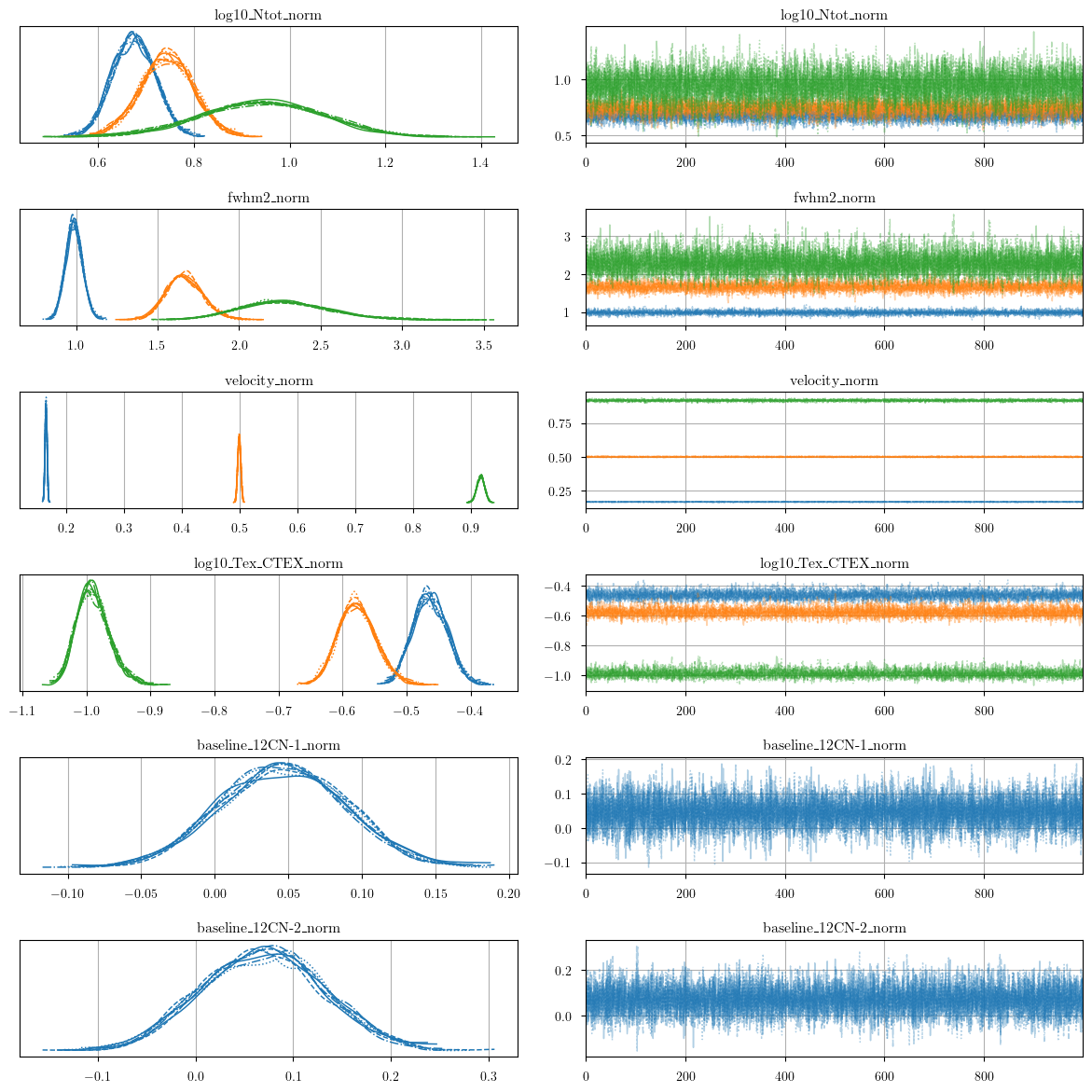
We generate posterior predictive checks as well as a trace plot of the individual chains. In the posterior predictive plot, we show each chain as a different color. Each line is one posterior sample.
[21]:
posterior = model.sample_posterior_predictive(
    thin=10, # keep one in {thin} posterior samples
)
_ = plot_predictive(model.data, posterior.posterior_predictive)
Sampling: [12CN-1, 12CN-2]
[22]:
from bayes_spec.plots import plot_traces

axes = plot_traces(model.trace.solution_0, model.cloud_freeRVs + model.baseline_freeRVs + model.hyper_freeRVs)
fig = axes.ravel()[0].figure
fig.tight_layout()
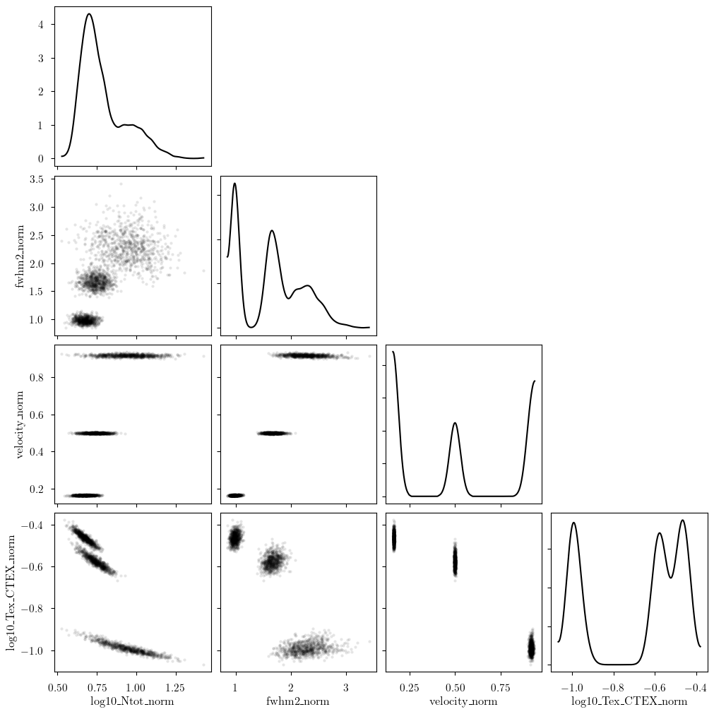
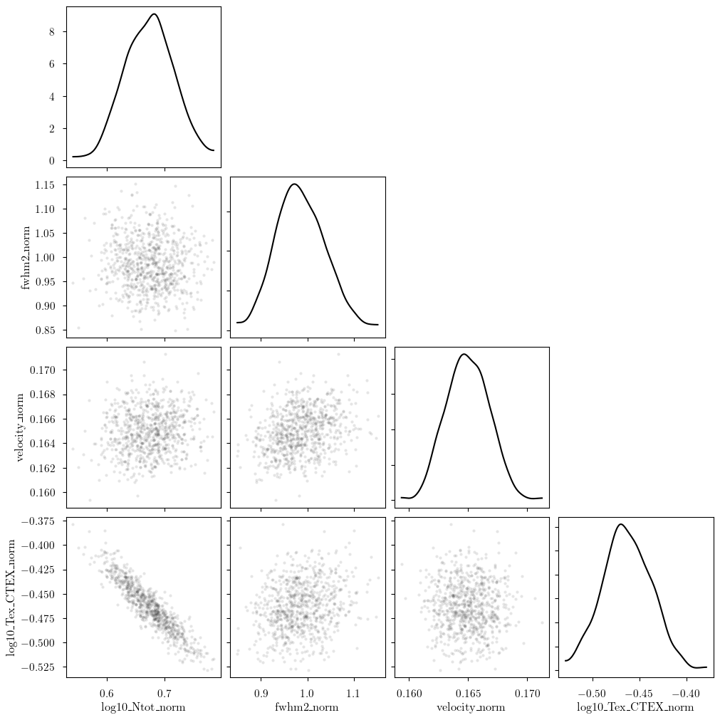
We can inspect the posterior distribution pair plots. First, the free parameters for all clouds. Keep an eye out for any strong degeneracies or non-linear correlations. If present, then these features can cause the posterior sampling to be inefficient. It may be worth re-parameterizing your model to remove these effects. Alternatively, increasing tune and target_accept can help.
[23]:
var_names = [
    param for param in model.cloud_freeRVs
    if not set(model.model.named_vars_to_dims[param]).intersection(set(["transition", "state"]))
]
print(var_names)
_ = plot_pair(
    model.trace.solution_0.sel(draw=slice(None, None, 10)), # samples
    var_names, # var_names to plot
    combine_dims=["cloud"], # concatenate clouds
    kind="scatter", # plot type
)
['log10_Ntot_norm', 'fwhm2_norm', 'velocity_norm', 'log10_Tex_CTEX_norm']
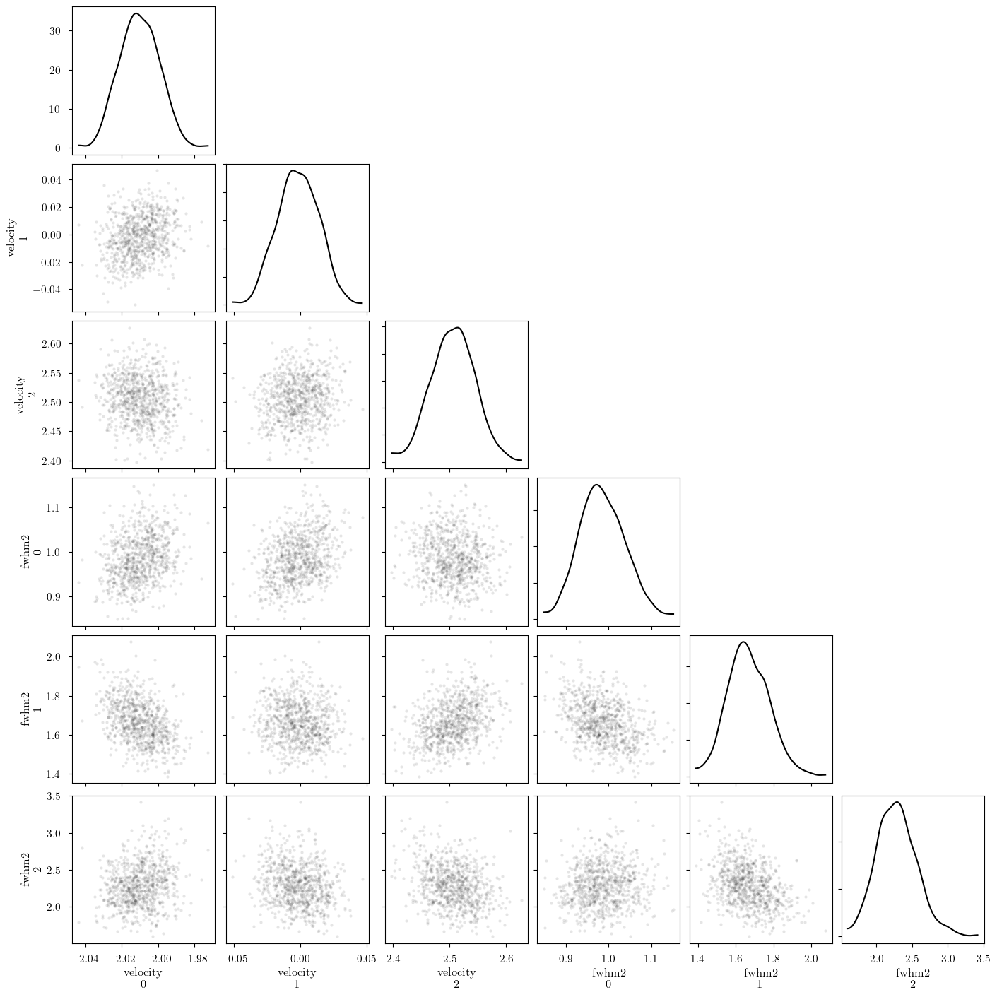
[24]:
_ = plot_pair(
    model.trace.solution_0.sel(draw=slice(None, None, 10)), # samples
    ["velocity", "fwhm2"], # var_names to plot
    combine_dims=None, # do not concatenate clouds
    kind="scatter", # plot type
)
[25]:
_ = plot_pair(
    model.trace.solution_0.sel(cloud=0, draw=slice(None, None, 10)), # samples
    var_names, # var_names to plot
    kind="scatter", # plot type
)
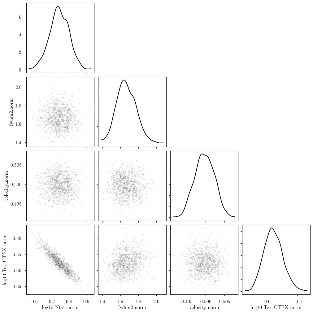
[26]:
_ = plot_pair(
    model.trace.solution_0.sel(cloud=1, draw=slice(None, None, 10)), # samples
    var_names, # var_names to plot
    kind="scatter", # plot type
)
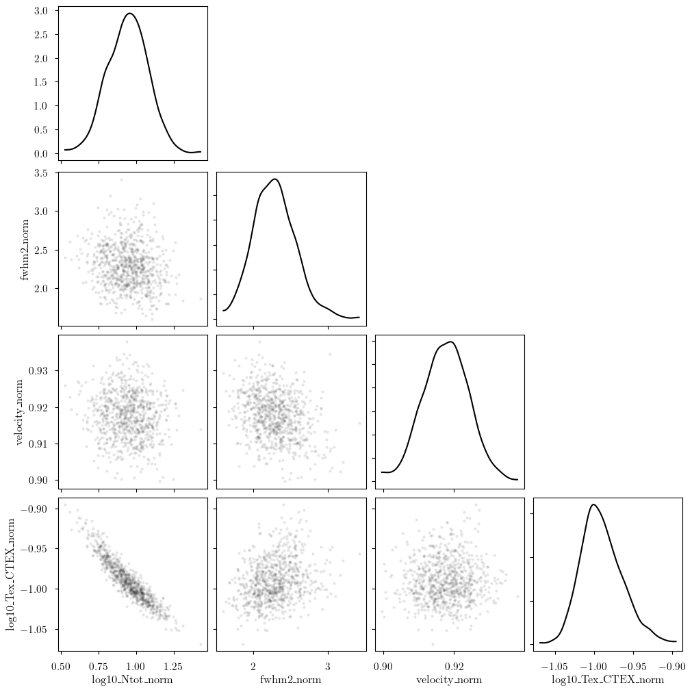
[27]:
_ = plot_pair(
    model.trace.solution_0.sel(cloud=2, draw=slice(None, None, 10)), # samples
    var_names, # var_names to plot
    kind="scatter", # plot type
)
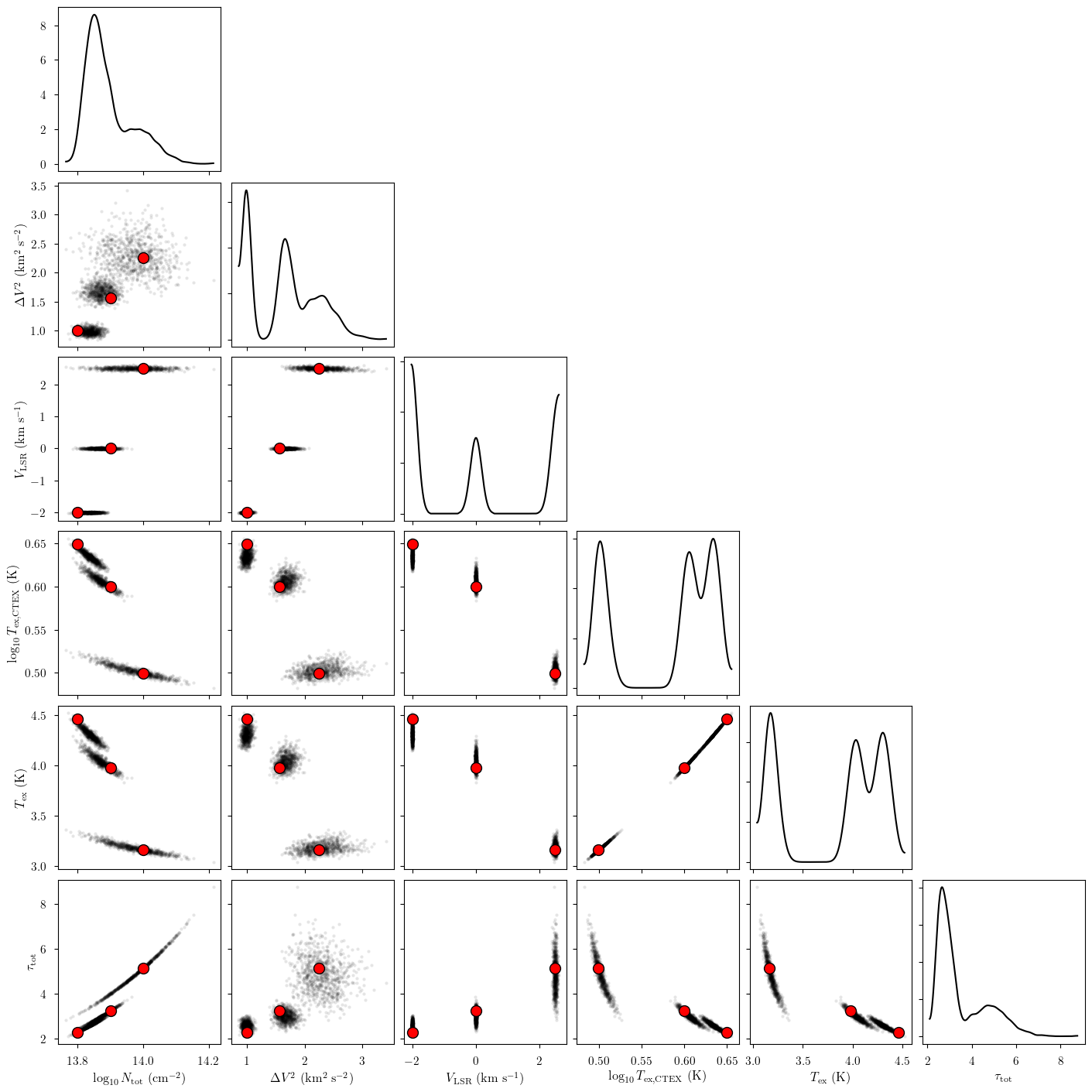
The red points represent the simulation parameters for the deterministic quantities.
[28]:
var_names = [
    param for param in model.cloud_deterministics + [p for p in model.cloud_freeRVs if "_norm" not in p]
    if not set(model.model.named_vars_to_dims[param]).intersection(set(["transition", "state"]))
]
print(var_names)

_ = plot_pair(
    model.trace.solution_0.sel(draw=slice(None, None, 10)), # samples
    var_names, # var_names to plot
    combine_dims=["cloud"], # concatenate clouds
    labeller=model.labeller, # label manager
    kind="scatter", # plot type
    reference_values=sim_params, # truths
)
['log10_Ntot', 'fwhm2', 'velocity', 'log10_Tex_CTEX', 'Tex', 'tau_total']
[29]:
# identify simulation cloud corresponding to each posterior cloud
sim_cloud_map = {}
for i in range(n_clouds):
    posterior_velocity = model.trace.solution_0['velocity'].sel(cloud=i).data.mean()
    match = np.argmin(np.abs(sim_params["velocity"] - posterior_velocity))
    sim_cloud_map[i] = match
sim_cloud_map
[29]:
{0: np.int64(0), 1: np.int64(1), 2: np.int64(2)}
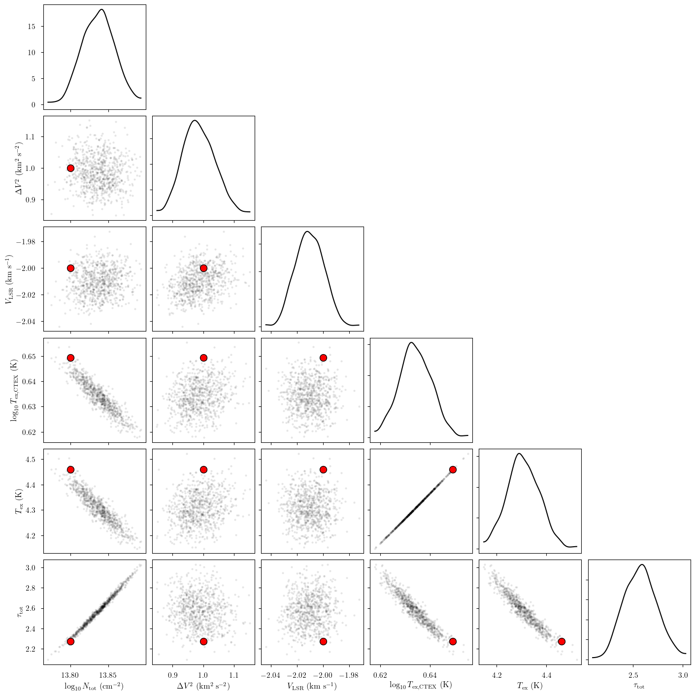
[30]:
cloud = 0

# subset of sim_params
my_sim_params = {}
for var_name in var_names:
    my_sim_params[var_name] = sim_params[var_name][sim_cloud_map[cloud]]

_ = plot_pair(
    model.trace.solution_0.sel(cloud=cloud, draw=slice(None, None, 10)), # samples
    var_names, # var_names to plot
    labeller=model.labeller, # label manager
    kind="scatter", # plot type
    reference_values=my_sim_params, # truths
)
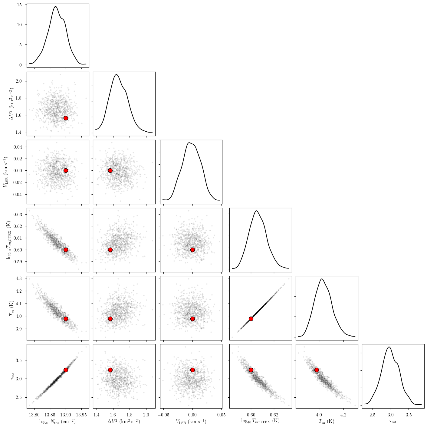
[31]:
cloud = 1

# subset of sim_params
my_sim_params = {}
for var_name in var_names:
    my_sim_params[var_name] = sim_params[var_name][sim_cloud_map[cloud]]

_ = plot_pair(
    model.trace.solution_0.sel(cloud=cloud, draw=slice(None, None, 10)), # samples
    var_names, # var_names to plot
    labeller=model.labeller, # label manager
    kind="scatter", # plot type
    reference_values=my_sim_params, # truths
)
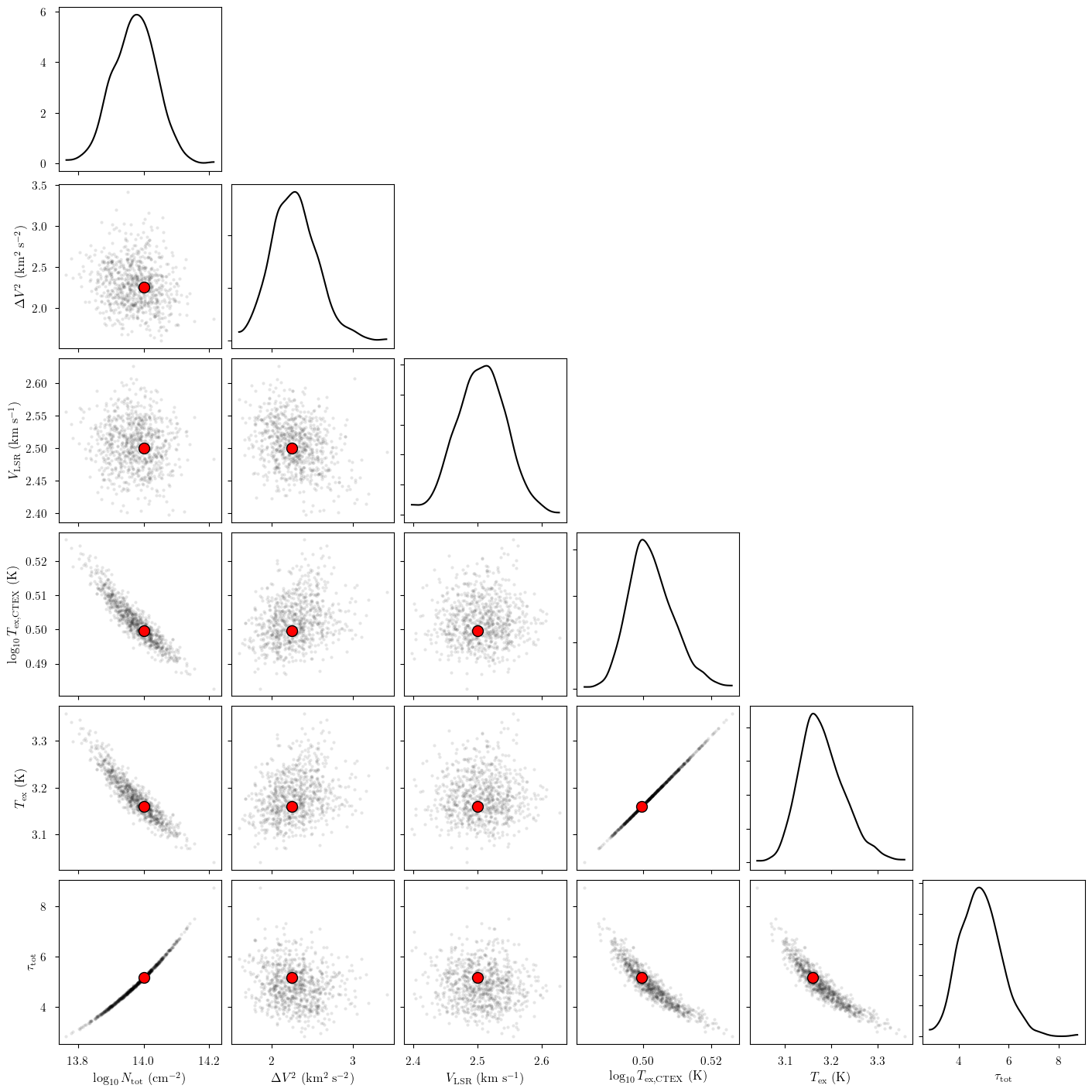
[32]:
cloud = 2

# subset of sim_params
my_sim_params = {}
for var_name in var_names:
    my_sim_params[var_name] = sim_params[var_name][sim_cloud_map[cloud]]

_ = plot_pair(
    model.trace.solution_0.sel(cloud=cloud, draw=slice(None, None, 10)), # samples
    var_names, # var_names to plot
    labeller=model.labeller, # label manager
    kind="scatter", # plot type
    reference_values=my_sim_params, # truths
)
Finally, we can get the posterior statistics, Bayesian Information Criterion (BIC), etc.
[33]:
point_stats = az.summary(model.trace.solution_0, kind='stats')
print("BIC:", model.bic())
display(point_stats)
BIC: -3413.0028007805786
| mean | sd | hdi_3% | hdi_97% | |
|---|---|---|---|---|
| baseline_12CN-1_norm[0] | 0.046 | 0.043 | -0.031 | 0.130 |
| baseline_12CN-2_norm[0] | 0.069 | 0.062 | -0.050 | 0.180 |
| log10_Ntot_norm[0] | 0.675 | 0.044 | 0.589 | 0.752 |
| log10_Ntot_norm[1] | 0.743 | 0.055 | 0.640 | 0.849 |
| log10_Ntot_norm[2] | 0.942 | 0.128 | 0.701 | 1.183 |
| log10_Tex_CTEX_norm[0] | -0.463 | 0.027 | -0.512 | -0.415 |
| log10_Tex_CTEX_norm[1] | -0.577 | 0.030 | -0.635 | -0.522 |
| log10_Tex_CTEX_norm[2] | -0.989 | 0.026 | -1.035 | -0.940 |
| fwhm2_norm[0] | 0.988 | 0.051 | 0.894 | 1.085 |
| fwhm2_norm[1] | 1.666 | 0.112 | 1.464 | 1.881 |
| fwhm2_norm[2] | 2.285 | 0.273 | 1.781 | 2.799 |
| velocity_norm[0] | 0.165 | 0.002 | 0.162 | 0.168 |
| velocity_norm[1] | 0.500 | 0.003 | 0.494 | 0.504 |
| velocity_norm[2] | 0.918 | 0.007 | 0.905 | 0.930 |
| log10_Ntot[0] | 13.837 | 0.022 | 13.794 | 13.876 |
| log10_Ntot[1] | 13.872 | 0.028 | 13.820 | 13.925 |
| log10_Ntot[2] | 13.971 | 0.064 | 13.851 | 14.091 |
| fwhm2[0] | 0.988 | 0.051 | 0.894 | 1.085 |
| fwhm2[1] | 1.666 | 0.112 | 1.464 | 1.881 |
| fwhm2[2] | 2.285 | 0.273 | 1.781 | 2.799 |
| velocity[0] | -2.010 | 0.011 | -2.029 | -1.990 |
| velocity[1] | -0.003 | 0.016 | -0.033 | 0.025 |
| velocity[2] | 2.506 | 0.039 | 2.432 | 2.578 |
| log10_Tex_CTEX[0] | 0.634 | 0.007 | 0.622 | 0.646 |
| log10_Tex_CTEX[1] | 0.606 | 0.007 | 0.591 | 0.619 |
| log10_Tex_CTEX[2] | 0.503 | 0.006 | 0.491 | 0.515 |
| CTEX_weights[0, 0 0 1 1 -- --] | 2.000 | 0.000 | 2.000 | 2.000 |
| CTEX_weights[0, 0 0 1 2 -- --] | 4.000 | 0.000 | 4.000 | 4.000 |
| CTEX_weights[0, 1 0 1 1 -- --] | 0.567 | 0.011 | 0.547 | 0.587 |
| CTEX_weights[0, 1 0 1 2 -- --] | 1.133 | 0.022 | 1.093 | 1.173 |
| CTEX_weights[0, 1 0 2 1 -- --] | 0.565 | 0.011 | 0.544 | 0.585 |
| CTEX_weights[0, 1 0 2 2 -- --] | 1.129 | 0.022 | 1.089 | 1.169 |
| CTEX_weights[0, 1 0 2 3 -- --] | 1.694 | 0.033 | 1.634 | 1.754 |
| CTEX_weights[1, 0 0 1 1 -- --] | 2.000 | 0.000 | 1.999 | 2.000 |
| CTEX_weights[1, 0 0 1 2 -- --] | 4.000 | 0.000 | 4.000 | 4.000 |
| CTEX_weights[1, 1 0 1 1 -- --] | 0.521 | 0.012 | 0.497 | 0.543 |
| CTEX_weights[1, 1 0 1 2 -- --] | 1.041 | 0.024 | 0.994 | 1.085 |
| CTEX_weights[1, 1 0 2 1 -- --] | 0.518 | 0.012 | 0.495 | 0.540 |
| CTEX_weights[1, 1 0 2 2 -- --] | 1.037 | 0.024 | 0.990 | 1.081 |
| CTEX_weights[1, 1 0 2 3 -- --] | 1.555 | 0.036 | 1.486 | 1.622 |
| CTEX_weights[2, 0 0 1 1 -- --] | 1.999 | 0.000 | 1.999 | 1.999 |
| CTEX_weights[2, 0 0 1 2 -- --] | 4.000 | 0.000 | 4.000 | 4.000 |
| CTEX_weights[2, 1 0 1 1 -- --] | 0.363 | 0.009 | 0.346 | 0.380 |
| CTEX_weights[2, 1 0 1 2 -- --] | 0.725 | 0.018 | 0.692 | 0.760 |
| CTEX_weights[2, 1 0 2 1 -- --] | 0.361 | 0.009 | 0.344 | 0.378 |
| CTEX_weights[2, 1 0 2 2 -- --] | 0.722 | 0.018 | 0.688 | 0.756 |
| CTEX_weights[2, 1 0 2 3 -- --] | 1.083 | 0.028 | 1.033 | 1.135 |
| Tex[0] | 4.307 | 0.066 | 4.187 | 4.430 |
| Tex[1] | 4.035 | 0.069 | 3.902 | 4.163 |
| Tex[2] | 3.182 | 0.047 | 3.095 | 3.271 |
| tau[113123.3701, 0] | 0.031 | 0.002 | 0.027 | 0.035 |
| tau[113123.3701, 1] | 0.036 | 0.003 | 0.031 | 0.042 |
| tau[113123.3701, 2] | 0.059 | 0.009 | 0.041 | 0.076 |
| tau[113144.1573, 0] | 0.255 | 0.017 | 0.224 | 0.286 |
| tau[113144.1573, 1] | 0.296 | 0.024 | 0.250 | 0.340 |
| tau[113144.1573, 2] | 0.479 | 0.077 | 0.338 | 0.623 |
| tau[113170.4915, 0] | 0.249 | 0.016 | 0.218 | 0.279 |
| tau[113170.4915, 1] | 0.289 | 0.023 | 0.244 | 0.332 |
| tau[113170.4915, 2] | 0.468 | 0.075 | 0.330 | 0.609 |
| tau[113191.2787, 0] | 0.323 | 0.021 | 0.284 | 0.362 |
| tau[113191.2787, 1] | 0.375 | 0.030 | 0.317 | 0.432 |
| tau[113191.2787, 2] | 0.608 | 0.098 | 0.429 | 0.791 |
| tau[113488.1202, 0] | 0.324 | 0.021 | 0.285 | 0.364 |
| tau[113488.1202, 1] | 0.377 | 0.030 | 0.318 | 0.433 |
| tau[113488.1202, 2] | 0.610 | 0.098 | 0.430 | 0.793 |
| tau[113490.9702, 0] | 0.861 | 0.057 | 0.756 | 0.966 |
| tau[113490.9702, 1] | 1.000 | 0.081 | 0.845 | 1.151 |
| tau[113490.9702, 2] | 1.620 | 0.260 | 1.143 | 2.107 |
| tau[113499.6443, 0] | 0.256 | 0.017 | 0.225 | 0.287 |
| tau[113499.6443, 1] | 0.297 | 0.024 | 0.251 | 0.342 |
| tau[113499.6443, 2] | 0.481 | 0.077 | 0.339 | 0.626 |
| tau[113508.9074, 0] | 0.250 | 0.016 | 0.219 | 0.280 |
| tau[113508.9074, 1] | 0.290 | 0.023 | 0.245 | 0.334 |
| tau[113508.9074, 2] | 0.470 | 0.075 | 0.332 | 0.611 |
| tau[113520.4315, 0] | 0.031 | 0.002 | 0.027 | 0.035 |
| tau[113520.4315, 1] | 0.036 | 0.003 | 0.031 | 0.042 |
| tau[113520.4315, 2] | 0.059 | 0.009 | 0.041 | 0.077 |
| tau_total[0] | 2.578 | 0.169 | 2.265 | 2.894 |
| tau_total[1] | 2.997 | 0.242 | 2.532 | 3.448 |
| tau_total[2] | 4.852 | 0.779 | 3.424 | 6.314 |
| TR[113123.3701, 0] | 2.149 | 0.058 | 2.043 | 2.256 |
| TR[113123.3701, 1] | 1.912 | 0.060 | 1.798 | 2.023 |
| TR[113123.3701, 2] | 1.204 | 0.037 | 1.136 | 1.275 |
| TR[113144.1573, 0] | 2.148 | 0.058 | 2.043 | 2.256 |
| TR[113144.1573, 1] | 1.911 | 0.060 | 1.797 | 2.022 |
| TR[113144.1573, 2] | 1.204 | 0.037 | 1.136 | 1.274 |
| TR[113170.4915, 0] | 2.148 | 0.058 | 2.042 | 2.255 |
| TR[113170.4915, 1] | 1.911 | 0.060 | 1.797 | 2.022 |
| TR[113170.4915, 2] | 1.204 | 0.037 | 1.136 | 1.274 |
| TR[113191.2787, 0] | 2.148 | 0.058 | 2.042 | 2.255 |
| TR[113191.2787, 1] | 1.911 | 0.060 | 1.797 | 2.022 |
| TR[113191.2787, 2] | 1.204 | 0.037 | 1.136 | 1.274 |
| TR[113488.1202, 0] | 2.143 | 0.058 | 2.038 | 2.251 |
| TR[113488.1202, 1] | 1.907 | 0.060 | 1.793 | 2.017 |
| TR[113488.1202, 2] | 1.200 | 0.037 | 1.132 | 1.270 |
| TR[113490.9702, 0] | 2.143 | 0.058 | 2.038 | 2.251 |
| TR[113490.9702, 1] | 1.907 | 0.060 | 1.793 | 2.017 |
| TR[113490.9702, 2] | 1.200 | 0.037 | 1.132 | 1.270 |
| TR[113499.6443, 0] | 2.143 | 0.058 | 2.038 | 2.251 |
| TR[113499.6443, 1] | 1.906 | 0.060 | 1.792 | 2.017 |
| TR[113499.6443, 2] | 1.200 | 0.037 | 1.132 | 1.270 |
| TR[113508.9074, 0] | 2.143 | 0.058 | 2.038 | 2.251 |
| TR[113508.9074, 1] | 1.906 | 0.060 | 1.792 | 2.017 |
| TR[113508.9074, 2] | 1.200 | 0.037 | 1.132 | 1.270 |
| TR[113520.4315, 0] | 2.143 | 0.058 | 2.037 | 2.250 |
| TR[113520.4315, 1] | 1.906 | 0.060 | 1.792 | 2.017 |
| TR[113520.4315, 2] | 1.200 | 0.037 | 1.132 | 1.270 |
[ ]: